You're here because you're serious about becoming a data analyst. You’ve probably noticed that just about every data analytics job posting asks for experience. But how do individuals get experience if they’re just starting out?! The answer: you do it by building a solid portfolio of data analytic projects so that you can land a job as a junior data analyst, even with no experience.

Your portfolio is your ticket to proving your capabilities to a potential employer. Even without previous job experience, a well-curated collection of data analytics projects can set you apart from the competition. They demonstrate your ability to tackle real-world problems with real data, showcasing your ability to clean datasets, create compelling visualizations, and extract meaningful insights—skills that are in high demand.

You just have to pick the ones that speak to you and get started!

Getting started with data analytics projects

So, you're ready to tackle your first data analytics project? Awesome! Let's break down what you need to know to set yourself up for success.

Our curated list of 20 projects below will help you develop the most sought-after data analysis skills and practice using the most frequently used data analysis tools. Namely:

• Python
• R
• Microsoft Excel
• Tableau
• Power BI
• SQL

Setting up an effective development environment is also vital. Begin by creating a Python environment with Conda or venv. Use version control like Git to track project changes. Combine an IDE like Jupyter Notebook with core Python libraries to boost your productivity.

Remember, Rome wasn't built in a day! Start your data analysis journey with bite-sized projects to steadily build your skills. Keep learning, stay curious, and enjoy the ride. Before you know it, you'll be tackling real-world data challenges like the professionals do.

Each project listed below will help you apply what you've learned to real data, growing your abilities one step at a time. While they are tailored towards beginners, some will be more challenging than others. By working through them, you'll create a portfolio that shows a potential employer you have the practical skills to analyze data on the job.

The data analytics projects below cover a range of analysis techniques, applications, and tools:

1. Learn and Install Jupyter Notebook
2. Profitable App Profiles for the App Store and Google Play Markets
3. Exploring Hacker News Posts
4. Clean and Analyze Employee Exit Surveys
5. Star Wars Survey
6. Word Raider
7. Install RStudio
8. Creating An Efficient Data Analysis Workflow
9. Creating An Efficient Data Analysis Workflow, Part 2
10. Preparing Data with Excel
11. Visualizing the Answer to Stock Questions Using Spreadsheet Charts
12. Identifying Customers Likely to Churn for a Telecommunications Provider
13. Data Prep in Tableau
14. Business Intelligence Plots
15. Data Presentation
16. Modeling Data in Power BI
17. Visualization of Life Expectancy and GDP Variation Over Time
18. Building a BI App
19. Analyzing Kickstarter Projects
20. Analyzing Startup Fundraising Deals from Crunchbase

In the following sections, you'll find step-by-step guides to walk you through each project. These detailed instructions will help you apply what you've learned and solidify your data analytics skills.

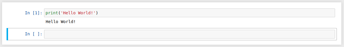
1. Learn and Install Jupyter Notebook

Overview

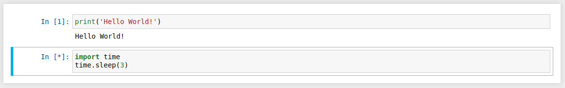
In this beginner-level project, you'll assume the role of a Jupyter Notebook novice aiming to gain the essential skills for real-world data analytics projects. You'll practice running code cells, documenting your work with Markdown, navigating Jupyter using keyboard shortcuts, mitigating hidden state issues, and installing Jupyter locally. By the end of the project, you'll be equipped to use Jupyter Notebook to work on data analytics projects and share compelling, reproducible notebooks with others.

Tools and Technologies

• Jupyter Notebook
• Python

Prerequisites

Before you take on this project, it's recommended that you have some foundational Python skills in place first, such as:

• Working with Python variables and data types
• Manipulating Python lists and dictionaries
• Writing Python functions

Step-by-Step Instructions

1. Get acquainted with the Jupyter Notebook interface and its components
2. Practice running code cells and learn how execution order affects results
3. Use keyboard shortcuts to efficiently navigate and edit notebooks
4. Create Markdown cells to document your code and communicate your findings
5. Install Jupyter locally to work on projects on your own machine

Expected Outcomes

Upon completing this project, you'll have gained practical experience and valuable skills, including:

• Familiarity with the core components and workflow of Jupyter Notebook
• Ability to use Jupyter Notebook to run code, perform analysis, and share results
• Understanding of how to structure and document notebooks for real-world reproducibility
• Proficiency in navigating Jupyter Notebook using keyboard shortcuts to boost productivity
• Readiness to apply Jupyter Notebook skills to real-world data projects and collaborate with others

Relevant Links and Resources

• How to Use Jupyter Notebook: A Beginner's Tutorial

Additional Resources

• 28 Jupyter Notebook Tips, Tricks, and Shortcuts
• Tutorial: Advanced Jupyter Notebooks

2. Profitable App Profiles for the App Store and Google Play Markets

Overview

In this guided project, you'll assume the role of a data analyst for a company that builds ad-supported mobile apps. By analyzing historical data from the Apple App Store and Google Play Store, you'll identify app profiles that attract the most users and generate the most revenue. Using Python and Jupyter Notebook, you'll clean the data, analyze it using frequency tables and averages, and make practical recommendations on the app categories and characteristics the company should target to maximize profitability.

Tools and Technologies

• Python
• Data Analytics
• Jupyter Notebook

Prerequisites

This is a beginner-level project, but you should be comfortable working with Python functions and Jupyter Notebook:

• Writing functions with arguments, return statements, and control flow
• Debugging functions to ensure proper execution
• Using conditional logic and loops within functions
• Working with Jupyter Notebook to write and run code

Step-by-Step Instructions

1. Open and explore the App Store and Google Play datasets
2. Clean the datasets by removing non-English apps and duplicate entries
3. Isolate the free apps for further analysis
4. Determine the most common app genres and their characteristics using frequency tables
5. Make recommendations on the ideal app profiles to maximize users and revenue

Expected Outcomes

By completing this project, you'll gain practical experience and valuable skills, including:

• Cleaning real-world data to prepare it for analysis
• Analyzing app market data to identify trends and success factors
• Applying data analysis techniques like frequency tables and calculating averages
• Using data insights to inform business strategy and decision-making
• Communicating your findings and recommendations to stakeholders

Relevant Links and Resources

• Python Functions and Jupyter Notebook course
• How to Use Jupyter Notebook: A Beginner's Tutorial

Additional Resources

• Basic Data Science Portfolio Project Tutorial
• Dataquest community where you can view and share this project with others
• Example Solution Code

3. Exploring Hacker News Posts

Overview

In this project, you'll explore and analyze a dataset from Hacker News, a popular tech-focused community site. Using Python, you'll apply skills in string manipulation, object-oriented programming, and date management to uncover trends in user submissions and identify factors that drive community engagement. This hands-on project will strengthen your ability to interpret real-world datasets and enhance your data analysis skills.

Tools and Technologies

• Python
• Data cleaning
• Object-oriented programming
• Data Analytics
• Jupyter Notebook

Prerequisites

To get the most out of this project, you should have some foundational Python and data cleaning skills, such as:

• Employing loops in Python to explore CSV data
• Utilizing string methods in Python to clean data for analysis
• Processing dates from strings using the datetime library
• Formatting dates and times for analysis using strftime

Step-by-Step Instructions

1. Remove headers from a list of lists
2. Extract 'Ask HN' and 'Show HN' posts
3. Calculate the average number of comments for 'Ask HN' and 'Show HN' posts
4. Find the number of 'Ask HN' posts and average comments by hour created
5. Sort and print values from a list of lists

Expected Outcomes

After completing this project, you'll have gained practical experience and skills, including:

• Applying Python string manipulation, OOP, and date handling to real-world data
• Analyzing trends and patterns in user submissions on Hacker News
• Identifying factors that contribute to post popularity and engagement
• Communicating insights derived from data analysis

Relevant Links and Resources

• Data Analyst in Python
• Original Hacker News Posts dataset on Kaggle
• Hacker News

Additional Resources

• Dataquest community where you can view and share this project with others
• Example Solution Code

4. Clean and Analyze Employee Exit Surveys

Overview

In this hands-on project, you'll play the role of a data analyst for the Department of Education, Training and Employment (DETE) and the Technical and Further Education (TAFE) institute in Queensland, Australia. Your task is to clean and analyze employee exit surveys from both institutes to identify insights into why employees resign. Using Python and pandas, you'll combine messy data from multiple sources, clean column names and values, analyze the data, and share your key findings.

Tools and Technologies

• Python
• Pandas
• Data cleaning
• Data Analytics
• Jupyter Notebook

Prerequisites

Before starting this project, you should be familiar with:

• Exploring and analyzing data using pandas
• Aggregating data with pandas groupby operations
• Combining datasets using pandas concat and merge functions
• Manipulating strings and handling missing data in pandas

Step-by-Step Instructions

1. Load and explore the DETE and TAFE exit survey data
2. Identify missing values and drop unnecessary columns
3. Clean and standardize column names across both datasets
4. Filter the data to only include resignation reasons
5. Verify data quality and create new columns for analysis
6. Combine the cleaned datasets into one for further analysis
7. Analyze the cleaned data to identify trends and insights

Expected Outcomes

By completing this project, you will:

• Clean real-world, messy HR data to prepare it for analysis
• Apply core data cleaning techniques in Python and pandas
• Combine multiple datasets and conduct exploratory analysis
• Analyze employee exit surveys to understand key drivers of resignations
• Summarize your findings and share data-driven recommendations

Relevant Links and Resources

• Pandas and NumPy Fundamentals Course

Additional Resources

• Community Feedback on Guided Project
• Example Solution Code

5. Star Wars Survey

Overview

In this project designed for beginners, you'll become a data analyst exploring FiveThirtyEight's Star Wars survey data. Using Python and pandas, you'll clean messy data, map values, compute statistics, and analyze the data to uncover fan film preferences. By comparing results between demographic segments, you'll gain insights into how Star Wars fans differ in their opinions. This project provides hands-on practice with key data cleaning and analysis techniques essential for data analyst roles across industries.

Tools and Technologies

• Python
• Pandas
• Jupyter Notebook

Prerequisites

Before starting this project, you should be familiar with the following:

• Exploring and cleaning data using pandas
• Combining datasets and performing joins in pandas
• Applying functions over columns in pandas DataFrames
• Analyzing survey data using pandas

Step-by-Step Instructions

1. Map Yes/No columns to Boolean values to standardize the data
2. Convert checkbox columns to lists and get them into a consistent format
3. Clean and rename the ranking columns to make them easier to analyze
4. Identify the highest-ranked and most-viewed Star Wars films
5. Analyze the data by key demographic segments like gender, age, and location
6. Summarize your findings on fan preferences and differences between groups

Expected Outcomes

After completing this project, you will have gained:

• Experience cleaning and analyzing a real-world, messy dataset
• Hands-on practice with pandas data manipulation techniques
• Insights into the preferences and opinions of Star Wars fans
• An understanding of how to analyze survey data for business insights

Relevant Links and Resources

• FiveThirtyEight's Star Wars Survey Data
• Introduction to Python Programming

Additional Resources

• Dataquest Community - Star Wars Survey Project
• Example Solution Code

6. Word Raider

Overview

In this beginner-level Python project, you'll step into the role of a developer to create "Word Raider," an interactive word-guessing game. Although this project won't have you perform any explicit data analysis, it will sharpen your Python skills and make you a better data analyst. Using fundamental programming skills, you'll apply concepts like loops, conditionals, and file handling to build the game logic from the ground up. This hands-on project allows you to consolidate your Python knowledge by integrating key techniques into a fun application.

Tools and Technologies

• Python
• Jupyter Notebook

Prerequisites

Before diving into this project, you should have some foundational Python skills, including:

• Familiarity with Python basics like variables, data types, and functions
• Ability to work with loops and conditional statements to control program flow
• Experience with reading data from files and manipulating strings
• Basic understanding of object-oriented programming concepts

Step-by-Step Instructions

1. Build the word bank by reading words from a text file into a Python list
2. Set up variables to track the game state, like the hidden word and remaining attempts
3. Implement functions to receive and validate user input for their guesses
4. Create the game loop, checking guesses against the hidden word and providing feedback
5. Update the game state after each guess and check for a win or loss condition

Expected Outcomes

By completing this project, you'll gain practical experience and valuable skills, including:

• Strengthened proficiency in fundamental Python programming concepts
• Experience building an interactive, text-based game from scratch
• Practice with file I/O, data structures, and basic object-oriented design
• Improved problem-solving skills and ability to translate ideas into code

Relevant Links and Resources

• Junior Data Analyst career path
• How to Become a Junior Data Analyst in 2024

Additional Resources

• Dataquest Community: My Take on the Word Raider Game
• Selecting and Installing an IDE
• Example Solution Code

7. Install RStudio

Overview

In this beginner-level project, you'll take the first steps in your data analysis journey by installing R and RStudio. As an aspiring data analyst, you'll set up a professional programming environment and explore RStudio's features for efficient R coding and analysis. Through guided exercises, you'll write scripts, import data, and create visualizations, building key foundations for your career.

Tools and Technologies

• R
• RStudio

Prerequisites

To complete this project, it's recommended to have basic knowledge of:

• R syntax and programming fundamentals
• Variables, data types, and arithmetic operations in R
• Logical and relational operators in R expressions
• Importing, exploring, and visualizing datasets in R

Step-by-Step Instructions

1. Install the latest version of R and RStudio on your computer
2. Practice writing and executing R code in the Console
3. Import a dataset into RStudio and examine its contents
4. Write and save R scripts to organize your code
5. Generate basic data visualizations using ggplot2

Expected Outcomes

By completing this project, you'll gain essential skills including:

• Setting up an R development environment with RStudio
• Navigating RStudio's interface for data science workflows
• Writing and running R code in scripts and the Console
• Installing and loading R packages for analysis and visualization
• Importing, exploring, and visualizing data in RStudio

Relevant Links and Resources

• R Basics for Data Analysis
• The Comprehensive R Archive Network

Additional Resources

• Top Tips for Learning R from Africa R’s Shelmith Kariuki
• The most trusted IDE for open source data science

8. Creating An Efficient Data Analysis Workflow

Overview

In this hands-on project, you'll step into the role of a data analyst hired by a company selling programming books. Your mission is to analyze their sales data to determine which titles are most profitable. You'll apply key R programming concepts like control flow, loops, and functions to develop an efficient data analysis workflow. This project provides valuable practice in data cleaning, transformation, and analysis, culminating in a structured report of your findings and recommendations.

Tools and Technologies

• R
• RStudio
• Data Analytics

Prerequisites

To successfully complete this project, you should have the following foundational control flow, iteration, and functions in R skills:

• Implementing control flow using if-else statements
• Employing for loops and while loops for iteration
• Writing custom functions to modularize code
• Combining control flow, loops, and functions in R

Step-by-Step Instructions

1. Get acquainted with the provided book sales dataset
2. Transform and prepare the data for analysis
3. Analyze the cleaned data to identify top performing titles
4. Summarize your findings in a structured report
5. Provide data-driven recommendations to stakeholders

Expected Outcomes

By completing this project, you'll gain practical experience and valuable skills, including:

• Applying R programming concepts to real-world data analysis
• Developing an efficient, reproducible data analysis workflow
• Cleaning and preparing messy data for analysis
• Analyzing sales data to derive actionable business insights
• Communicating findings and recommendations to stakeholders

Relevant Links and Resources

• Getting Started with R and RStudio - Dataquest Blog
• Download the Book Reviews dataset - CSV file

Additional Resources

• Example Solution Code
• Dataquest community where you can view and share this project with others

9. Creating An Efficient Data Analysis Workflow, Part 2

Overview

In this hands-on project, you'll step into the role of a data analyst at a book company tasked with evaluating the impact of a new program launched on July 1, 2019 to encourage customers to buy more books. Using your data analysis skills in R, you'll clean and process the company's 2019 sales data to determine if the program successfully boosted book purchases and improved review quality. This project allows you to apply key R packages like dplyr, stringr, and lubridate to efficiently analyze a real-world business dataset and deliver actionable insights.

Tools and Technologies

• R
• RStudio
• dplyr
• stringr
• lubridate

Prerequisites

To successfully complete this project, you should have some specialized data processing in R skills:

• Manipulating strings using stringr functions
• Working with dates and times using lubridate
• Applying the map function to vectorize custom functions
• Understanding and employing regular expressions for pattern matching

Step-by-Step Instructions

1. Load and explore the book company's 2019 sales data
2. Clean the data by handling missing values and inconsistencies
3. Process the text reviews to determine positive/negative sentiment
4. Compare key sales metrics like purchases and revenue before and after the July 1 program launch date
5. Analyze differences in sales between customer segments

Expected Outcomes

By completing this project, you'll gain practical experience and valuable skills, including:

• Cleaning and preparing a real-world business dataset for analysis
• Applying powerful R packages to manipulate and process data efficiently
• Analyzing sales data to quantify the impact of a new initiative
• Translating analysis findings into meaningful business insights

Relevant Links and Resources

• Download the Book Sales dataset - CSV file
• Data Analyst in R Path

Additional Resources

• Example Solution Code
• Dataquest community where you can view and share this project with others

10. Preparing Data with Excel

Overview

In this hands-on project for beginners, you'll step into the role of a data professional in a marine biology research organization. Your mission is to prepare a raw dataset on shark attacks for an analysis team to study trends in attack locations and frequency over time. Using Excel, you'll import the data, organize it in worksheets and tables, handle missing values, and clean the data by removing duplicates and fixing inconsistencies. This project provides practical experience in the essential data preparation skills required for real-world analysis projects.

Tools and Technologies

• Excel

Prerequisites

This project is designed for beginners. To complete it, you should be familiar with preparing data in Excel:

• Importing data into Excel from various sources
• Organizing spreadsheet data using worksheets and tables
• Cleaning data by removing duplicates, fixing inconsistencies, and handling missing values
• Consolidating data from multiple sources into a single table

Step-by-Step Instructions

1. Import the raw shark attack data into an Excel workbook
2. Organize the data into worksheets and tables with a logical structure
3. Clean the data by removing duplicate entries and fixing inconsistencies
4. Consolidate shark attack data from multiple sources into a single table

Expected Outcomes

By completing this project, you will gain:

• Hands-on experience in data preparation and cleaning techniques using Excel
• Foundational skills for importing, organizing, and cleaning data for analysis
• An understanding of how to handle missing values and inconsistencies in a dataset
• Ability to consolidate data from disparate sources into an analysis-ready format
• Practical experience working with a real-world dataset on shark attacks
• A solid foundation for data analysis projects and further learning in Excel

Relevant Links and Resources

• Shark attacks dataset - Kaggle
• Introduction to Data Analysis with Excel Skill Path

Additional Resources

• Dataquest community where you can view and share this project with others

11. Visualizing the Answer to Stock Questions Using Spreadsheet Charts

Overview

In this hands-on project, you'll step into the shoes of a business analyst to explore historical stock market data using Excel. By applying information design concepts, you'll create compelling visualizations and craft an insightful report – building valuable skills for communicating data-driven insights that are highly sought-after by employers across industries.

Tools and Technologies

• Excel
• Data visualization
• Information design principles

Prerequisites

To successfully complete this project, it's recommended to have foundational visualizing data in Excel skills, such as:

• Creating various chart types in Excel to visualize data
• Selecting appropriate chart types to effectively present data
• Applying design principles to create clear and informative charts
• Designing charts for an audience using Gestalt principles

Step-by-Step Instructions

1. Import the dataset to an Excel spreadsheet
2. Create a report using data visualizations and tabular data
3. Represent the data using effective data visualizations
4. Apply Gestalt principles and pre-attentive attributes to all visualizations
5. Maximize data-ink ratio in all visualizations

Expected Outcomes

By completing this project, you'll gain practical experience and valuable skills, including:

• Analyzing real-world stock market data in Excel
• Applying information design principles to create effective visualizations
• Selecting the best chart types to answer specific questions about the data
• Combining multiple charts into a cohesive, insightful report
• Developing in-demand data visualization and communication skills

Relevant Links and Resources

• Microsoft Stock Data - Kaggle
• Amazon Stock Data - Kaggle
• INTEL Stock Data - Kaggle
• Bitcoin Historical Data - Kaggle
• Introduction to Data Analysis with Excel Skill Path

Additional Resources

• Dataquest community where you can view and share this project with others

12. Identifying Customers Likely to Churn for a Telecommunications Provider

Overview

In this beginner project, you'll take on the role of a data analyst at a telecommunications company. Your challenge is to explore customer data in Excel to identify profiles of those likely to churn. Retaining customers is crucial for telecom providers, so your insights will help inform proactive retention efforts. You'll conduct exploratory data analysis, calculating key statistics, building PivotTables to slice the data, and creating charts to visualize your findings. This project provides hands-on experience with core Excel skills for data-driven business decisions that will enhance your analyst portfolio.

Tools and Technologies

• Excel

Prerequisites

To complete this project, you should feel comfortable exploring data in Excel:

• Calculating descriptive statistics in Excel
• Analyzing data with descriptive statistics
• Creating PivotTables in Excel to explore and analyze data
• Visualizing data with histograms and boxplots in Excel

Step-by-Step Instructions

1. Import the customer dataset into Excel
2. Calculate descriptive statistics for key metrics
3. Create PivotTables, histograms, and boxplots to explore data differences
4. Analyze and identify profiles of likely churners
5. Compile a report with your data visualizations

Expected Outcomes

By completing this project, you'll gain practical experience and valuable skills, including:

• Hands-on practice analyzing a real-world customer dataset in Excel
• Ability to calculate and interpret key statistics to profile churn risks
• Experience building PivotTables and charts to slice data and uncover insights
• Skill in translating analysis findings into an actionable report for stakeholders

Relevant Links and Resources

• Customer Churn Prediction 2020 dataset - Kaggle
• Introduction to Data Analysis with Excel Skill Path

Additional Resources

• Dataquest community where you can view and share this project with others

13. Data Prep in Tableau

Overview

In this hands-on project, you'll take on the role of a data analyst for Dataquest to prepare their online learning platform data for analysis. You'll connect to Excel data, import tables into Tableau, and define table relationships to build a data model for uncovering insights on student engagement and performance. This project focuses on essential data preparation steps in Tableau, providing you with a robust foundation for data visualization and analysis.

Tools and Technologies

• Tableau

Prerequisites

To successfully complete this project, you should have some foundational skills in preparing data in Tableau, such as:

• Connecting to data sources in Tableau to access the required data
• Importing data tables into the Tableau canvas
• Defining relationships between tables in Tableau to combine data
• Cleaning and filtering imported data in Tableau to prepare it for use

Step-by-Step Instructions

1. Connect to the provided Excel file containing key tables on student engagement, course performance, and content completion rates
2. Import the tables into Tableau and define the relationships between tables to create a unified data model
3. Clean and filter the imported data to handle missing values, inconsistencies, or irrelevant information
4. Save the prepared data source to use for creating visualizations and dashboards
5. Reflect on the importance of proper data preparation for effective analysis

Expected Outcomes

By completing this project, you will gain valuable skills and experience, including:

• Hands-on practice with essential data preparation techniques in Tableau
• Ability to connect to, import, and combine data from multiple tables
• Understanding of how to clean and structure data for analysis
• Readiness to progress to creating visualizations and dashboards to uncover insights

Relevant Links and Resources

• Download the dataset - Excel (xlsx) file
• Data Visualization with Tableau Skill Path

Additional Resources

• Tableau Community Forums
• Tableau Documentation

14. Business Intelligence Plots

Overview

In this hands-on project, you'll step into the role of a data visualization consultant for Adventure Works. The company's leadership team wants to understand the differences between their online and offline sales channels. You'll apply your Tableau skills to build insightful, interactive data visualizations that provide clear comparisons and enable data-driven business decisions. Key techniques include creating calculated fields, applying filters, utilizing dual-axis charts, and embedding visualizations in tooltips. By the end, you'll have a set of powerful Tableau dashboards ready to share with stakeholders.

Tools and Technologies

• Tableau

Prerequisites

To successfully complete this project, you should have a solid grasp of data visualization fundamentals in Tableau:

• Navigating the Tableau interface and distinguishing between dimensions and measures
• Constructing various foundational chart types in Tableau
• Developing and interpreting calculated fields to enhance analysis
• Employing filters to improve visualization interactivity

Step-by-Step Instructions

1. Compare online vs offline orders using visualizations
2. Analyze products across channels with scatter plots
3. Embed visualizations in tooltips for added insight
4. Summarize findings and identify next steps

Expected Outcomes

Upon completing this project, you'll have gained valuable skills and experience:

• Practical experience building interactive business intelligence dashboards in Tableau
• Ability to create calculated fields to conduct tailored analysis
• Understanding of how to use filters and tooltips to enable data exploration
• Skill in developing visualizations that surface actionable insights for stakeholders

Relevant Links and Resources

• Data Visualization with Tableau Skill Path

Additional Resources

• Tableau Community Forums
• Tableau Documentation

15. Data Presentation

Overview

In this project, you'll step into the role of a data analyst exploring conversion funnel trends for a company's leadership team. Using Tableau, you'll build interactive dashboards that uncover insights about which marketing channels, locations, and customer personas drive the most value in terms of volume and conversion rates. By applying data visualization best practices and incorporating dashboard actions and filters, you'll create a professional, usable dashboard ready to present your findings to stakeholders.

Tools and Technologies

• Tableau

Prerequisites

To successfully complete this project, you should be comfortable sharing insights in Tableau, such as:

• Building basic charts like bar charts and line graphs in Tableau
• Employing color, size, trend lines and forecasting to emphasize insights
• Combining charts, tables, text and images into dashboards
• Creating interactive dashboards with filters and quick actions

Step-by-Step Instructions

1. Import and clean the conversion funnel data in Tableau
2. Build basic charts to visualize key metrics
3. Create interactive dashboards with filters and actions
4. Add annotations and highlights to emphasize key insights
5. Compile a professional dashboard to present findings

Expected Outcomes

Upon completing this project, you'll have gained practical experience and valuable skills, including:

• Analyzing conversion funnel data to surface actionable insights
• Visualizing trends and comparisons using Tableau charts and graphs
• Applying data visualization best practices to create impactful dashboards
• Adding interactivity to enable exploration of the data
• Communicating data-driven findings and recommendations to stakeholders

Relevant Links and Resources

• Data Visualization with Tableau Skill Path
• Example Solution

Additional Resources

• Tableau Community Forums
• Tableau Documentation

16. Modeling Data in Power BI

Overview

In this hands-on project, you'll step into the role of an analyst at a company that sells scale model cars. Your mission is to model and analyze data from their sales records database using Power BI to extract insights that drive business decision-making. Power BI is a powerful business analytics tool that enables you to connect to, model, and visualize data. By applying data cleaning, transformation, and modeling techniques in Power BI, you'll prepare the sales data for analysis and develop practical skills in working with real-world datasets. This project provides valuable experience in extracting meaningful insights from raw data to inform business strategy.

Tools and Technologies

• Power BI

Prerequisites

To successfully complete this project, you should know how to model data in Power BI, such as:

• Designing a basic data model in Power BI
• Configuring table and column properties in Power BI
• Creating calculated columns and measures using DAX in Power BI
• Reviewing the performance of measures, relationships, and visuals in Power BI

Step-by-Step Instructions

1. Import the sales data into Power BI
2. Clean and transform the data for analysis
3. Design a basic data model in Power BI
4. Create calculated columns and measures using DAX
5. Build visualizations to extract insights from the data

Expected Outcomes

Upon completing this project, you'll have gained valuable skills and experience, including:

• Hands-on practice modeling and analyzing real-world sales data in Power BI
• Ability to clean, transform and prepare data for analysis
• Experience extracting meaningful business insights from raw data
• Developing practical skills in data modeling and analysis using Power BI

Relevant Links and Resources

• Introduction to Power BI
• Official Power BI documentation

Additional Resources

• Power BI Community
• A CEO Explains How to Learn Power BI (Step-By-Step)

17. Visualization of Life Expectancy and GDP Variation Over Time

Overview

In this project, you'll step into the role of a data analyst tasked with visualizing life expectancy and GDP data over time to uncover trends and regional differences. Using Power BI, you'll apply data cleaning, transformation, and visualization skills to create interactive scatter plots and stacked column charts that reveal insights from the Gapminder dataset. This hands-on project allows you to practice the full life-cycle of report and dashboard development in Power BI. You'll load and clean data, create and configure visualizations, and publish your work to showcase your skills. By the end, you'll have an engaging, interactive dashboard to add to your portfolio.

Tools and Technologies

• Power BI

Prerequisites

To complete this project, you should be able to visualize data in Power BI, such as:

• Creating basic Power BI visuals
• Designing accessible report layouts
• Customizing report themes and visual markers
• Publishing Power BI reports and dashboards

Step-by-Step Instructions

1. Import the life expectancy and GDP data into Power BI
2. Clean and transform the data for analysis
3. Create interactive scatter plots and stacked column charts
4. Design an accessible report layout in Power BI
5. Customize visual markers and themes to enhance insights

Expected Outcomes

By completing this project, you'll gain practical experience and valuable skills, including:

• Applying data cleaning, transformation, and visualization techniques in Power BI
• Creating interactive scatter plots and stacked column charts to uncover data insights
• Developing an engaging dashboard to showcase your data visualization skills
• Practicing the full life-cycle of Power BI report and dashboard development

Relevant Links and Resources

• Introduction to Power BI
• Official Power BI Support
• Official Power BI documentation

Additional Resources

• Why Business Analysts Need to Learn Power BI

18. Building a BI App

Overview

In this hands-on project, you'll step into the role of a business intelligence analyst at Dataquest, an online learning platform. Using Power BI, you'll import and model data on course completion rates and Net Promoter Scores (NPS) to assess course quality. You'll create insightful visualizations like KPI metrics, line charts, and scatter plots to analyze trends and compare courses. Leveraging this analysis, you'll provide data-driven recommendations on which courses Dataquest should improve.

Tools and Technologies

• Power BI

Prerequisites

To successfully complete this project, you should have some foundational skills in Power BI, such as how to manage workspaces and datasets in Power BI:

• Creating and managing workspaces
• Importing and updating assets within a workspace
• Developing dynamic reports using parameters
• Implementing static and dynamic row-level security

Step-by-Step Instructions

1. Import and explore the course completion and NPS data, looking for data quality issues
2. Create a data model relating the fact and dimension tables
3. Write calculations for key metrics like completion rate and NPS, and validate the results
4. Design and build visualizations to analyze course performance trends and comparisons

Expected Outcomes

Upon completing this project, you'll have gained valuable skills and experience:

• Importing, modeling, and analyzing data in Power BI to drive decisions
• Creating calculated columns and measures to quantify key metrics
• Designing and building insightful data visualizations to convey trends and comparisons
• Developing impactful reports and dashboards to summarize findings
• Sharing data stories and recommending actions via Power BI apps

Relevant Links and Resources

• Introduction to Power BI
• Official Power BI documentation

Additional Resources

• What’s the best way to learn Microsoft Power BI?
• Sample datasets from Power BI

19. Analyzing Kickstarter Projects

Overview

In this hands-on project, you'll step into the role of a data analyst to explore and analyze Kickstarter project data using SQL. You'll start by importing and exploring the dataset, followed by cleaning the data to ensure accuracy. Then, you'll write SQL queries to uncover trends and insights within the data, such as success rates by category, funding goals, and more. By the end of this project, you'll be able to use SQL to derive meaningful insights from real-world datasets.

Tools and Technologies

• SQL

Prerequisites

To successfully complete this project, you should be comfortable working with SQL and databases, such as:

• Basic SQL commands and querying
• Data manipulation and joins in SQL
• Experience with cleaning data and handling missing values

Step-by-Step Instructions

1. Import and explore the Kickstarter dataset to understand its structure
2. Clean the data to handle missing values and ensure consistency
3. Write SQL queries to analyze the data and uncover trends
4. Visualize the results of your analysis using SQL queries

Expected Outcomes

Upon completing this project, you'll have gained valuable skills and experience, including:

• Proficiency in using SQL for data analysis
• Experience with cleaning and analyzing real-world datasets
• Ability to derive insights from Kickstarter project data

Relevant Links and Resources

• Original Dataset - Kaggle
• SQL Fundamentals skill path

Additional Resources

• SQL Joins Tutorial: Working with Databases

20. Analyzing Startup Fundraising Deals from Crunchbase

Overview

In this beginner-level guided project, you'll step into the role of a data analyst to explore a dataset of startup investments from Crunchbase. By applying your pandas and SQLite skills, you'll work with a large dataset to uncover insights on fundraising trends, successful startups, and active investors. This project focuses on developing techniques for handling memory constraints, selecting optimal data types, and leveraging SQL databases. You'll strengthen your ability to apply the pandas-SQLite workflow to real-world scenarios.

Tools and Technologies

• Python
• Pandas
• SQLite
• Jupyter Notebook

Prerequisites

Although this is a beginner-level SQL project, you'll need some solid skills in Python and data analysis before taking it on:

• Python fundamentals, including variables, data types, and basic syntax
• Familiarity with pandas for data manipulation and analysis
• Basics of data cleaning techniques to handle missing data and inconsistencies
• Exposure to SQL databases and querying data using SQLite

Step-by-Step Instructions

1. Explore the structure and contents of the Crunchbase startup investments dataset
2. Process the large dataset in chunks and load into an SQLite database
3. Analyze fundraising rounds data to identify trends and derive insights
4. Examine the most successful startup verticals based on total funding raised
5. Identify the most active investors by number of deals and total amount invested

Expected Outcomes

Upon completing this guided project, you'll gain practical skills and experience, including:

• Applying pandas and SQLite to analyze real-world startup investment data
• Handling large datasets effectively through chunking and efficient data types
• Integrating pandas DataFrames with SQL databases for scalable data analysis
• Deriving actionable insights from fundraising data to understand startup success
• Building a project for your portfolio showcasing pandas and SQLite skills

Relevant Links and Resources

• Data Analyst in Python career path
• SQL Fundamentals skill path

Additional Resources

• Dataquest Community Discussion on the Project
• SQL Commands: The Complete List (w/ Examples)

Choosing the right data analyst projects

Since the list of data analytics projects on the internet is exhaustive (and can be exhausting!), no one can be expected to build them all. So, how do you pick the right ones for your portfolio, whether they're guided or independent projects? Let's go over the criteria you should use to make this decision.

Passions vs. Interests vs. In-Demand skills

When selecting projects, it’s essential to strike a balance between your passions, interests, and in-demand skills. Here’s how to navigate these three factors:

• Passions: Choose projects that genuinely excite you and align with your long-term goals. Passions are often areas you are deeply committed to and are willing to invest significant time and effort in. Working on something you are passionate about can keep you motivated and engaged, which is crucial for learning and completing the project.
• Interests: Pick projects related to fields or a topic that sparks your curiosity or enjoyment. Interests might not have the same level of commitment as passions, but they can still make the learning process more enjoyable and meaningful. For instance, if you're curious about sports analytics or healthcare data, these interests can guide your project choices.
• In-Demand Skills: Focus on projects that help you develop skills currently sought after in the job market. Research job postings and industry trends to identify which skills are in demand and tailor your projects to develop those competencies.

Steps to picking the right data analytics projects

1. Assess your current skill level
   • If you’re a beginner, start with projects that focus on data cleaning (an essential skill), exploration, and visualization. Using Python libraries like Pandas and Matplotlib is an efficient way to build these foundational skills.
   • Utilize structured resources that provide both a beginner data analyst learning path and support to guide you through your first projects.
2. Plan before you code
   • Clearly define your topic, project objectives, and key questions upfront to stay focused and aligned with your goals.
   • Choose appropriate data sources early in the planning process to streamline the rest of the project.
3. Focus on the fundamentals
   • Clean your data thoroughly to ensure accuracy.
   • Use analytical techniques that align with your objectives.
   • Create clear, impactful visualizations of your findings.
   • Document your process for reproducibility and effective communication.
4. Start small and scale up
   • Begin with small, manageable projects to build your confidence and skills.
   • When you're ready, take on more challenging projects that use machine learning or web scraping, like Predicting Heart Disease or Web Scraping Football Matches.
5. Seek feedback and iterate
   • Share your projects with peers, mentors, or online communities to get feedback.
   • Use this feedback to improve and refine your work.

Remember, it’s okay to start small and gradually take on bigger challenges. Each project you complete, no matter how simple, helps you gain skills and learn valuable lessons. Tackling a series of focused projects is one of the best ways to grow your abilities as a data professional. With each one, you’ll get better at planning, execution, and communication.

Conclusion

If you're serious about landing a data analytics job, project-based learning is key.

There’s a lot of data out there and a lot you can do with it. Trying to figure out where to start can be overwhelming. If you want a more structured approach to reaching your goal, consider enrolling in Dataquest’s Data Analyst in Python career path. It offers exactly what you need to land your first job as a data analyst or to grow your career by adding one of the most popular programming languages, in-demand data skills, and projects to your CV.

But if you’re confident in doing this on your own, the list of projects we’ve shared in this post will definitely help you get there. To continue improving, we encourage you to take on additional projects and share them in the Dataquest Community. This provides valuable peer feedback, helping you refine your projects to become more advanced and join the group of professionals who do this for a living.

Completing Python projects is the ultimate way to learn the language. When you work on real-world projects, you not only retain more of the lessons you learn, but you'll also find it super motivating to push yourself to pick up new skills. Because let's face it, no one actually enjoys sitting in front of a screen learning random syntax for hours on end―particularly if it's not going to be used right away.

Python projects don't have this problem. Anything new you learn will stick because you're immediately putting it into practice. There's just one problem: many Python learners struggle to come up with their own Python project ideas to work on. But that's okay, we can help you with that!

Are You Ready for This?

If you have some programming experience, you might be ready to jump straight into building a Python project. However, if you’re just starting out, it’s vital you have a solid foundation in Python before you take on any projects. Otherwise, you run the risk of getting frustrated and giving up before you even get going. For those in need, we recommend taking either:

1. Introduction to Python Programming course: meant for those looking to become a data professional while learning the fundamentals of programming with Python.
   • This course is part of the Data Analyst in Python career path
2. Introduction to Python Programming course: meant for those looking to leverage the power of AI while learning the fundamentals of programming with Python.
   • This course is part of the Generative AI Fundamentals in Python skill path

In both courses, the goal is to quickly learn the basics of Python so you can start working on a project as soon as possible. You'll learn by doing, not by passively watching videos.

Selecting a Project

Our list below has 60+ fun and rewarding Python projects for learners at all levels. Some are free guided projects that you can complete directly in your browser via the Dataquest platform. Others are more open-ended, serving as inspiration as you build your Python skills. The key is to choose a project that resonates with you and just go for it!

Now, let’s take a look at some Python project examples. There is definitely something to get you started in this list.

Free Python Projects (Recommended):

These free Dataquest guided projects are a great place to start. They provide an embedded code editor directly in your browser, step-by-step instructions to help you complete the project, and community support if you happen to get stuck.

1. Building an Interactive Word Game — In this guided project, you’ll use basic Python programming concepts to create a functional and interactive word-guessing game.

2. Profitable App Profiles for the App Store and Google Play Markets — In this one, you’ll work as a data analyst for a company that builds mobile apps. You’ll use Python to analyze real app market data to find app profiles that attract the most users.

3. Exploring Hacker News Posts — Use Python string manipulation, OOP, and date handling to analyze trends driving post popularity on Hacker News, a popular technology site.

4. Learn and Install Jupyter Notebook — A guide to using and setting up Jupyter Notebook locally to prepare you for real-world data projects.

5. Predicting Heart Disease — We're tasked with using a dataset from the World Health Organization to accurately predict a patient’s risk of developing heart disease based on their medical data.

6. Analyzing Accuracy in Data Presentation — In this project, we'll step into the role of data journalists to analyze movie ratings data and determine if there’s evidence of bias in Fandango’s rating system.

Table of Contents

More Projects to Help Build Your Portfolio:

7. Finding Heavy Traffic Indicators on I-94 — Explore how using the pandas plotting functionality along with the Jupyter Notebook interface allows us to analyze data quickly using visualizations to determine indicators of heavy traffic.

8. Storytelling Data Visualization on Exchange Rates — You'll assume the role of a data analyst tasked with creating an explanatory data visualization about Euro exchange rates to inform and engage an audience.

9. Clean and Analyze Employee Exit Surveys — Work with exit surveys from employees of the Department of Education in Queensland, Australia. Play the role of a data analyst to analyze employee exit surveys and uncover insights about why employees resign.

10. Star Wars Survey — In this data cleaning project, you’ll work with Jupyter Notebook to analyze data on the Star Wars movies to answer the hotly contested question, "Who shot first?"

11. Analyzing NYC High School Data — For this project, you’ll assume the role of a data scientist analyzing relationships between SAT scores and demographic factors in NYC public schools to determine if the SAT is a fair test.

12. Predicting the Weather Using Machine Learning — For this project, you’ll step into the role of a data scientist to predict tomorrow’s weather using historical data and machine learning, developing skills in data preparation, time series analysis, and model evaluation.

13. Credit Card Customer Segmentation — For this project, we’ll play the role of a data scientist at a credit card company to segment customers into groups using K-means clustering in Python, allowing the company to tailor strategies for each segment.

Python Projects for AI Enthusiasts:

14. Building an AI Chatbot with Streamlit — Build a simple website with an AI chatbot user interface similar to the OpenAI Playground in this intermediate-level project using Streamlit.

15. Developing a Dynamic AI Chatbot — Create your very own AI-powered chatbot that can take on different personalities, keep track of conversation history, and provide coherent responses in this intermediate-level project.

16. Building a Food Ordering App — Create a functional application using Python dictionaries, loops, and functions to create an interactive system for viewing menus, modifying carts, and placing orders.

Table of Contents

Fun Python Projects for Building Data Skills:

17. Exploring eBay Car Sales Data — Use Python to work with a scraped dataset of used cars from eBay Kleinanzeigen, a classifieds section of the German eBay website.

18. Find out How Much Money You’ve Spent on Amazon — Dig into your own spending habits with this beginner-level tutorial!

19. Analyze Your Personal Netflix Data — Another beginner-to-intermediate tutorial that gets you working with your own personal dataset.

20. Analyze Your Personal Facebook Data with Python — Are you spending too much time posting on Facebook? The numbers don’t lie, and you can find them in this beginner-to-intermediate Python project.

21. Analyze Survey Data — This walk-through will show you how to set up Python and how to filter survey data from any dataset (or just use the sample data linked in the article).

22. All of Dataquest’s Guided Projects — These guided data science projects walk you through building real-world data projects of increasing complexity, with suggestions for how to expand each project.

23. Analyze Everything — Grab a free dataset that interests you, and start poking around! If you get stuck or aren’t sure where to start, our introduction to Python lessons are here to help, and you can try them for free!

Table of Contents

Cool Python Projects for Game Devs:

24. Rock, Paper, Scissors — Learn Python with a simple-but-fun game that everybody knows.

25. Build a Text Adventure Game — This is a classic Python beginner project (it also pops up in this book) that’ll teach you many basic game setup concepts that are useful for more advanced games.

26. Guessing Game — This is another beginner-level project that’ll help you learn and practice the basics.

27. Mad Libs — Use Python code to make interactive Python Mad Libs!

28. Hangman — Another childhood classic that you can make to stretch your Python skills.

29. Snake — This is a bit more complex, but it’s a classic (and surprisingly fun) game to make and play.

Simple Python Projects for Web Devs:

30. URL shortener — This free video course will show you how to build your own URL shortener like Bit.ly using Python and Django.

31. Build a Simple Web Page with Django — This is a very in-depth, from-scratch tutorial for building a website with Python and Django, complete with cartoon illustrations!

Easy Python Projects for Aspiring Developers:

32. Password generator — Build a secure password generator in Python.

33. Use Tweepy to create a Twitter bot — This Python project idea is a bit more advanced, as you’ll need to use the Twitter API, but it’s definitely fun!

34. Build an Address Book — This could start with a simple Python dictionary or become as advanced as something like this!

35. Create a Crypto App with Python — This free video course walks you through using some APIs and Python to build apps with cryptocurrency data.

Table of Contents

Additional Python Project Ideas

Still haven’t found a project idea that appeals to you? Here are many more, separated by experience level.

These aren’t tutorials; they’re just Python project ideas that you’ll have to dig into and research on your own, but that’s part of the fun! And it’s also part of the natural process of learning to code and working as a programmer.

The pros use Google and AI tools for answers all the time — so don’t be afraid to dive in and get your hands dirty!

Beginner Python Project Ideas

36. Create a text encryption generator. This would take text as input, replaces each letter with another letter, and outputs the “encoded” message.

37. Build a countdown calculator. Write some code that can take two dates as input, and then calculate the amount of time between them. This will be a great way to familiarize yourself with Python’s datetime module.

38. Write a sorting method. Given a list, can you write some code that sorts it alphabetically, or numerically? Yes, Python has this functionality built-in, but see if you can do it without using the sort() function!

39. Build an interactive quiz application. Which Avenger are you? Build a personality or recommendation quiz that asks users some questions, stores their answers, and then performs some kind of calculation to give the user a personalized result based on their answers

40. Tic-Tac-Toe by Text. Build a Tic-Tac-Toe game that’s playable like a text adventure. Can you make it print a text-based representation of the board after each move?

41. Make a temperature/measurement converter. Write a script that can convert Fahrenheit (℉) to Celcius (℃) and back, or inches to centimeters and back, etc. How far can you take it?

42. Build a counter app. Take your first steps into the world of UI by building a very simple app that counts up by one each time a user clicks a button.

43. Build a number-guessing game. Think of this as a bit like a text adventure, but with numbers. How far can you take it?

44. Build an alarm clock. This is borderline beginner/intermediate, but it’s worth trying to build an alarm clock for yourself. Can you create different alarms? A snooze function?

Table of Contents

Intermediate Python Project Ideas

45. Build an upgraded text encryption generator. Starting with the project mentioned in the beginner section, see what you can do to make it more sophisticated. Can you make it generate different kinds of codes? Can you create a “decoder” app that reads encoded messages if the user inputs a secret key? Can you create a more sophisticated code that goes beyond simple letter-replacement?

46. Make your Tic-Tac-Toe game clickable. Building off the beginner project, now make a version of Tic-Tac-Toe that has an actual UI  you’ll use by clicking on open squares. Challenge: can you write a simple “AI” opponent for a human player to play against?

47. Scrape some data to analyze. This could really be anything, from any website you like. The web is full of interesting data. If you learn a little about web-scraping, you can collect some really unique datasets.

48. Build a clock website. How close can you get it to real-time? Can you implement different time zone selectors, and add in the “countdown calculator” functionality to calculate lengths of time?

49. Automate some of your job. This will vary, but many jobs have some kind of repetitive process that you can automate! This intermediate project could even lead to a promotion.

50. Automate your personal habits. Do you want to remember to stand up once every hour during work? How about writing some code that generates unique workout plans based on your goals and preferences? There are a variety of simple apps you can build to automate or enhance different aspects of your life.

51. Create a simple web browser. Build a simple UI that accepts  URLs and loads webpages. PyWt will be helpful here! Can you add a “back” button, bookmarks, and other cool features?

52. Write a notes app. Create an app that helps people write and store notes. Can you think of some interesting and unique features to add?

53. Build a typing tester. This should show the user some text, and then challenge them to type it quickly and accurately. Meanwhile, you time them and score them on accuracy.

54. Create a “site updated” notification system. Ever get annoyed when you have to refresh a website to see if an out-of-stock product has been relisted? Or to see if any news has been posted? Write a Python script that automatically checks a given URL for updates and informs you when it identifies one. Be careful not to overload the servers of whatever site you’re checking, though. Keep the time interval reasonable between each check.

55. Recreate your favorite board game in Python. There are tons of options here, from something simple like Checkers all the way up to Risk. Or even more modern and advanced games like Ticket to Ride or Settlers of Catan. How close can you get to the real thing?

56. Build a Wikipedia explorer. Build an app that displays a random Wikipedia page. The challenge here is in the details: can you add user-selected categories? Can you try a different “rabbit hole” version of the app, wherein each article is randomly selected from the articles linked in the previous article? This might seem simple, but it can actually require some serious web-scraping skills.

Table of Contents

Advanced Python Project Ideas

57. Build a stock market prediction app. For this one, you’ll need a source of stock market data and some machine learning and data analytics skills. Fortunately, many people have tried this, so there’s plenty of source code out there to work from.

58. Build a chatbot. The challenge here isn’t so much making the chatbot as it is making it good. Can you, for example, implement some natural language processing techniques to make it sound more natural and spontaneous?

59. Program a robot. This requires some hardware (which isn’t usually free), but there are many affordable options out there — and many learning resources, too. Definitely look into Raspberry Pi if you’re not already thinking along those lines.

60. Build an image recognition app. Starting with handwriting recognition is a good idea — Dataquest has a guided data science project to help with that! Once you’ve learned it, you can take it to the next level.

61. Create a sentiment analysis tool for social media. Collect data from various social media platforms, preprocess it, and then train a deep learning model to analyze the sentiment of each post (positive, negative, neutral).

62. Make a price prediction model. Select an industry or product that interests you, and build a machine learning model that predicts price changes.

63. Create an interactive map. This will require a mix of data skills and UI creation skills. Your map can display whatever you’d like — bird migrations, traffic data, crime reports — but it should be interactive in some way. How far can you take it?

Table of Contents

Next Steps

Each of the examples in the previous sections built on the idea of choosing a great Python project for a beginner and then enhancing it as your Python skills progress. Next, you can advance to the following:

• Think about what interests you, and choose a project that overlaps with your interests.

• Think about your Python learning goals, and make sure your project moves you closer to achieving those goals.

• Start small. Once you’ve built a small project, you can either expand it or build another one.

Now you’re ready to get started. If you haven’t learned the basics of Python yet, I recommend diving in with Dataquest’s Introduction to Python Programming course.

If you already know the basics, there’s no reason to hesitate! Now is the time to get in there and find your perfect Python project.

Data is everywhere. Every click, purchase, or social media like creates mountains of information, but raw numbers do not tell a story. That is where data analysts come in. They turn messy datasets into actionable insights that help businesses grow.

Whether you're looking to become a junior data analyst or looking to level up, here are the top 11 data analyst skills every professional needs in 2025, including one optional skill that can help you stand out.

1. SQL

SQL (Structured Query Language) is the language of databases and is arguably the most important technical skill for analysts. It allows you to efficiently query and manage large datasets across multiple systems—something Excel cannot do at scale.

Example in action: Want last quarter's sales by region? SQL pulls it in seconds, no matter how huge the dataset.

Learning Tip: Start with basic queries, then explore joins, aggregations, and subqueries. Practicing data analytics exercises with SQL will help you build confidence and precision.

2. Excel

Since it’s not going anywhere, it’s still worth it to learn Microsoft Excel. Beyond spreadsheets, it offers pivot tables, macros, and Power Query, which are perfect for quick analysis on smaller datasets. Many startups or lean teams still rely on Excel as their first database.

Example in action: Summarize thousands of rows of customer feedback in minutes with pivot tables, then highlight trends visually.

Learning Tip: Focus on pivot tables, logical formulas, and basic automation. Once comfortable, try linking Excel to SQL queries or automating repetitive tasks to strengthen your technical skills in data analytics.

3. Python or R

Python and R are essential for handling big datasets, advanced analytics, and automation. Python is versatile for cleaning data, automation, and integrating analyses into workflows, while R excels at exploratory data analysis and statistical analysis.

Example in action: Clean hundreds of thousands of rows with Python’s pandas library in seconds, something that would take hours in Excel.

Learning Tip: Start with data cleaning and visualization, then move to complex analyses like regression or predictive modeling. Building these data analyst skills is critical for anyone working in data science. Of course, which is better to learn is still up for debate.

4. Data Visualization

Numbers alone rarely persuade anyone. Data visualization is how you make your insights clear and memorable. Tools like Tableau, Power BI, or Python/R libraries help you tell a story that anyone can understand.

Example in action: A simple line chart showing revenue trends can be far more persuasive than a table of numbers.

Learning Tip: Design visuals with your audience in mind. Recreate dashboards from online tutorials to practice clarity, storytelling, and your soft skills in communicating data analytics results.

5. Statistics & Analytics

Strong statistical analysis knowledge separates analysts who report numbers from those who generate insights. Skills like regression, correlation, hypothesis testing, and A/B testing help you interpret trends accurately.

Example in action: Before recommending a new marketing campaign, test whether the increase in sales is statistically significant or just random fluctuation.

Learning Tip: Focus on core probability and statistics concepts first, then practice applying them in projects. Our Probability and Statistics with Python skill path is a great way to learn theoretical concepts in a hands-on way.

6. Data Cleaning & Wrangling

Data rarely comes perfect, so data cleaning skills will always be in demand. Cleaning and transforming datasets, removing duplicates, handling missing values, and standardizing formats are often the most time-consuming but essential parts of the job.

Example in action: You want to analyze customer reviews, but ratings are inconsistent and some entries are blank. Cleaning the data ensures your insights are accurate and actionable.

Learning Tip: Practice on free datasets or public data repositories to build real-world data analyst skills.

7. Communication & Presentation Skills

Analyzing data is only half the battle. Sharing your findings clearly is just as important. Being able to present insights in reports, dashboards, or meetings ensures your work drives decisions.

Example in action: Presenting a dashboard to a marketing team that highlights which campaigns brought the most new customers can influence next-quarter strategy.

Learning Tip: Practice explaining complex findings to someone without a technical background. Focus on clarity, storytelling, and visuals rather than technical jargon. Strong soft skills are just as valuable as your technical skills in data analytics.

8. Dashboard & Report Creation

Beyond visualizations, analysts need to build dashboards and reports that allow stakeholders to interact with data. A dashboard is not just a fancy chart. It is a tool that empowers teams to make data-driven decisions without waiting for you to interpret every number.

Example in action: A sales dashboard with filters for region, product line, and time period can help managers quickly identify areas for improvement.

Learning Tip: Start with simple dashboards in Tableau, Power BI, or Google Data Studio. Focus on making them interactive, easy to understand, and aligned with business goals. This is an essential part of professional data analytics skills.

9. Domain Knowledge

Understanding the industry or context of your data makes you exponentially more effective. Metrics and trends mean different things depending on the business.

Example in action: Knowing e-commerce metrics like cart abandonment versus subscription churn metrics can change how you interpret the same type of data.

Learning Tip: Study your company’s industry, read case studies, or shadow colleagues in different departments to build context. The more you know, the better your insights and analysis will be.

10. Critical Thinking & Problem-Solving

Numbers can be misleading. Critical thinking lets analysts ask the right questions, identify anomalies, and uncover hidden insights.

Example in action: Revenue drops in one region. Critical thinking helps you ask whether it is seasonal, a data error, or a genuine trend.

Learning Tip: Challenge assumptions and always ask “why” multiple times when analyzing a dataset. Practice with open-ended case studies to sharpen your analytical thinking and overall data analyst skills.

11. Machine Learning Basics

Not every analyst uses machine learning daily, but knowing the basics—predictive modeling, clustering, or AI-powered insights—can help you stand out. You do not need this skill to get started as an analyst, but familiarity with it is increasingly valuable for advanced roles.

Example in action: Using a simple predictive model to forecast next month’s sales trends can help your team allocate resources more effectively.

Learning Tip: Start small with beginner-friendly tools like Python’s scikit-learn library, then explore more advanced models as you grow. Treat it as an optional skill to explore once you are confident in SQL, Python/R, and statistical analysis.

Where to Learn These Skills

Want to become a data analyst? Dataquest makes it easy to learn the skills you need to get hired.

With our Data Analyst in Python and Data Analyst in R career paths, you’ll learn by doing real projects, not just watching videos. Each course helps you build the technical and practical skills employers look for.

By the end, you’ll have the knowledge, experience, and confidence to start your career in data analysis.

Wrapping It Up

Being a data analyst is not just about crunching numbers. It is about turning data into actionable insights that drive decisions. Master these data analytics and data analyst skills, and you will be prepared to handle the challenges of 2025 and beyond.

If you've spent hours debugging a pandas KeyError, or writing the same data validation code for the hundredth time, or refactoring a messy analysis script, you know the frustration of tedious coding work. Real data science work involves analytical thinking and creative problem-solving, but it also requires a lot of mechanical coding: boilerplate writing, test generation, and documentation creation.

What if you could delegate the mechanical parts to an AI assistant that understands your codebase and handles implementation details while you focus on the analytical decisions?

That's what Claude Code does for data scientists.

What Is Claude Code?

Claude Code is Anthropic's terminal-based AI coding assistant that helps you write, refactor, debug, and document code through natural language conversations. Unlike autocomplete tools that suggest individual lines as you type, Claude Code understands project context, makes coordinated multi-file edits, and can execute workflows autonomously.

Claude Code excels at generating boilerplate code for data loading and validation, refactoring messy scripts into clean modules, debugging obscure errors in pandas or numpy operations, implementing standard patterns like preprocessing pipelines, and creating tests and documentation. However, it doesn't replace your analytical judgment, make methodological decisions about statistical approaches, or fix poorly conceived analysis strategies.

In this tutorial, you'll learn how to install Claude Code, understand its capabilities and limitations, and start using it productively for data science work. You'll see the core commands, discover tips that improve efficiency, and see concrete examples of how Claude Code handles common data science tasks.

Key Benefits for Data Scientists

Before we get into installation, let's establish what Claude Code actually does for data scientists:

1. Eliminate boilerplate code writing for repetitive patterns that consume time without requiring creative thought. File loading with error handling, data validation checks that verify column existence and types, preprocessing pipelines with standard transformations—Claude Code generates these in seconds rather than requiring manual implementation of logic you've written dozens of times before.
2. Generate test suites for data processing functions covering normal operation, edge cases with malformed or missing data, and validation of output characteristics. Testing data pipelines becomes straightforward rather than work you postpone.
3. Accelerate documentation creation for data analysis workflows by generating detailed docstrings, README files explaining project setup, and inline comments that explain complex transformations.
4. Debug obscure errors more efficiently in pandas operations, numpy array manipulations, or scikit-learn pipeline configurations. Claude Code interprets cryptic error messages, suggests likely causes based on common patterns, and proposes fixes you can evaluate immediately.
5. Refactor exploratory code into production-quality modules with proper structure, error handling, and maintainability standards. The transition from research notebook to deployable pipeline becomes faster and less painful.

These benefits translate directly to time savings on mechanical tasks, allowing you to focus on analysis, modeling decisions, and generating insights rather than wrestling with implementation details.

Installation and Setup

Let's get Claude Code installed and configured. The process takes about 10-15 minutes, including account creation and verification.

Step 1: Obtain Your Anthropic API Key

Navigate to console.anthropic.com and create an account if you don't have one. Once logged in, access the API keys section from the navigation menu on the left, and generate a new API key by clicking on + Create Key.

While you can generate a new key anytime from the console, you won’t be able to retrieve any existing API keys once they have been created. For this reason, you’ll want to copy your API key immediately and store it somewhere safe—you'll need it for authentication.

Always keep your API keys secure. Treat them like passwords and never commit them to version control or share them publicly.

Step 2: Install Claude Code

Claude Code installs via npm (Node Package Manager). If you don't have Node.js installed on your system, download it from nodejs.org before proceeding.

Once Node.js is installed, open your terminal and run:

npm install -g @anthropic-ai/claude-code

The -g flag installs Claude Code globally, making it available from any directory on your system.

Common installation issues:

• "npm: command not found": You need to install Node.js first. Download it from nodejs.org and restart your terminal after installation.
• Permission errors on Mac/Linux: Try sudo npm install -g @anthropic-ai/claude-code to install with administrator privileges.
• PATH issues: If Claude Code installs successfully but the claude command isn't recognized, you may need to add npm's global directory to your system PATH. Run npm config get prefix to find the location, then add [that-location]/bin to your PATH environment variable.

Step 3: Configure Authentication

Set your API key as an environment variable so Claude Code can authenticate with Anthropic's servers:

export ANTHROPIC_API_KEY=your_key_here

Replace your_key_here with the actual API key you copied earlier from the Anthropic console.

To make this permanent (so you don't need to set your API key every time you open a terminal), add the export line above to your shell configuration file:

• For bash: Add to ~/.bashrc or ~/.bash_profile
• For zsh: Add to ~/.zshrc
• For fish: Add to ~/.config/fish/config.fish

You can edit your shell configuration file using nano config_file_name. After adding the line, reload your configuration by running source ~/.bashrc (or whichever file you edited), or simply open a new terminal window.

Step 4: Verify Installation

Confirm that Claude Code is properly installed and authenticated:

claude --version

You should see version information displayed. If you get an error, review the installation steps above.

Try running Claude Code for the first time:

claude

This launches the Claude Code interface. You should see a welcome message and a prompt asking you to select the text style that looks best with your terminal:

Use the arrow keys on your keyboard to select a text style and press Enter to continue.

Next, you’ll be asked to select a login method:

If you have an eligible subscription, select option 1. Otherwise, select option 2. For this tutorial, we will use option 2 (API usage billing).

Once your account setup is complete, you’ll see a welcome message showing the email address for your account:

To exit the setup of Claude Code at any point, press Control+C twice.

Security Note

Claude Code can read files you explicitly include and generate code that loads data from files or databases. However, it doesn't automatically access your data without your instruction. You maintain full control over what files and information Claude Code can see. When working with sensitive data, be mindful of what files you include in conversation context and review all generated code before execution, especially code that connects to databases or external systems. For more details, see Anthropic’s Security Documentation.

Understanding the Costs

Claude Code itself is free software, but using it requires an Anthropic API key that operates on usage-based pricing:

• Free tier: Limited testing suitable for evaluation
• Pro plan (\$20/month): Reasonable usage for individual data scientists conducting moderate development work
• Pay-as-you-go: For heavy users working intensively on multiple projects, typically \$6-12 daily for active development

Most practitioners doing regular but not continuous development work find the \$20 Pro plan provides good balance between cost and capability. Start with the free tier to evaluate effectiveness on your actual work, then upgrade based on demonstrated value.

Your First Commands

Now that Claude Code is installed and configured, let's walk through basic usage with hands-on examples.

Starting a Claude Code Session

Navigate to a project directory in your terminal:

cd ~/projects/customer_analysis

Launch Claude Code:

claude

You'll see the Claude Code interface with a prompt where you can type natural language instructions.

Understanding Your Project

Before asking Claude Code to make changes, it needs to understand your project context. Try starting with this exploratory command:

Explain the structure of this project and identify the key files.

Claude Code will read through your directory, examine files, and provide a summary of what it found. This shows that Claude Code actively explores and comprehends codebases before acting.

Your First Refactoring Task

Let's demonstrate Claude Code's practical value with a realistic example. Create a simple file called load_data.py with some intentionally messy code:

import pandas as pd

# Load customer data
data = pd.read_csv('/Users/yourname/Desktop/customers.csv')
print(data.head())

This works but has obvious problems: hardcoded absolute path, no error handling, poor variable naming, and no documentation.

Now ask Claude Code to improve it:

Refactor load_data.py to use best practices: configurable paths, error handling, descriptive variable names, and complete docstrings.

Claude Code will analyze the file and propose improvements. Instead of the hardcoded path, you'll get configurable file paths through command-line arguments. The error handling expands to catch missing files, empty files, and CSV parsing errors. Variable names become descriptive (customer_df or customer_data instead of generic data). A complete docstring appears documenting parameters, return values, and potential exceptions. The function adds proper logging to track what's happening during execution.

Claude Code asks your permission before making these changes. Always review its proposal; if it looks good, approve it. If something seems off, ask for modifications or reject the changes entirely. This permission step ensures you stay in control while delegating the mechanical work.

What Just Happened

This demonstrates Claude Code's workflow:

1. You describe what you want in natural language
2. Claude Code analyzes the relevant files and context
3. Claude Code proposes specific changes with explanations
4. You review and approve or request modifications
5. Claude Code applies approved changes

The entire refactoring took 90 seconds instead of 20-30 minutes of manual work. More importantly, Claude Code caught details you might have forgotten, such as adding logging, proper type hints, and handling multiple error cases. The permission-based approach ensures you maintain control while delegating implementation work.

Core Commands and Patterns

Claude Code provides several slash (/) commands that control its behavior and help you work more efficiently.

Important Slash Commands

@filename: Reference files directly in your prompts using the @ symbol. Example: @src/preprocessing.py or Explain the logic in @data_loader.py. Claude Code automatically includes the file's content in context. Use tab completion after typing @ to quickly navigate and select files.

/clear: Reset conversation context entirely, removing all history and file references. Use this when switching between different analyses, datasets, or project areas. Accumulated conversation history consumes tokens and can cause Claude Code to inappropriately reference outdated context. Think of /clear as starting a fresh conversation when you switch tasks.

/help: Display available commands and usage information. Useful when you forget command syntax or want to discover capabilities.

Context Management for Data Science Projects

Claude Code has token limits determining how much code it can consider simultaneously. For small projects with a few files, this rarely matters. For larger data science projects with dozens of notebooks and scripts, strategic context management becomes important.

Reference only files relevant to your current task using @filename syntax. If you're working on data validation, reference the validation script and related utilities (like @validation.py and @utils/data_checks.py) but exclude modeling and visualization code that won't influence the current work.

Effective Prompting Patterns

Claude Code responds best to clear, specific instructions. Compare these approaches:

• Vague: "Make this code better"
  Specific: "Refactor this preprocessing function to handle missing values using median imputation for numerical columns and mode for categorical columns, add error handling for unexpected data types, and include detailed docstrings"
• Vague: "Add tests"
  Specific: "Create pytest tests for the data_loader function covering successful loading, missing file errors, empty file handling, and malformed CSV detection"
• Vague: "Fix the pandas error"
  Specific: "Debug the KeyError in line 47 of data_pipeline.py and suggest why it's failing on the 'customer_id' column"

Specific prompts produce focused, useful results. Vague prompts generate generic suggestions that may not address your actual needs.

Iteration and Refinement

Treat Claude Code's initial output as a starting point rather than expecting perfection on the first attempt. Review what it generates, identify improvements needed, and make follow-up requests:

"The validation function you created is good, but it should also check that dates are within reasonable ranges. Add validation that start_date is after 2000-01-01 and end_date is not in the future."

This iterative approach produces better results than attempting to specify every requirement in a single massive prompt.

Advanced Features

Beyond basic commands, several features improve your Claude Code experience for complex work.

1. Activate plan mode: Press Shift+Tab before sending your prompt to enable plan mode, which creates an explicit execution plan before implementing changes. Use this for workflows with three or more distinct steps—like loading data, preprocessing, and generating outputs. The planning phase helps Claude maintain focus on the overall objective.

2. Run commands with bash mode: Prefix prompts with an exclamation mark to execute shell commands and inject their output into Claude Code's context:

   ! python analyze_sales.py

   This runs your analysis script and adds complete output to Claude Code's context. You can then ask questions about the output or request interpretations of the results. This creates a tight feedback loop for iterative data exploration.

3. Use extended thinking for complex problems: Include "think", "think harder", or "ultrathink" in prompts for thorough analysis:

   think harder: why does my linear regression show high R-squared but poor prediction on validation data?

   Extended thinking produces more careful analysis but takes longer (ultrathink can take several minutes). Apply this when debugging subtle statistical issues or planning sophisticated transformations.

4. Resume previous sessions: Launch Claude Code with claude --resume to continue your most recent session with complete context preserved, including conversation history, file references, and established conventions all intact. This proves valuable for ongoing analysis where you want to continue today without re-explaining your entire analytical approach.

Optional Power User Setting

For personal projects where you trust all operations, launch with claude --dangerously-skip-permissions to bypass constant approval prompts. This carries risk if Claude Code attempts destructive operations, so use it only on projects where you maintain version control and can recover from mistakes. Never use this on production systems or shared codebases.

Configuring Claude Code for Data Science Projects

The CLAUDE.md file provides project-specific context that improves Claude Code's suggestions by explaining your conventions, requirements, and domain specifics.

Quick Setup with /init

The easiest way to create your CLAUDE.md file is using Claude Code's built-in /init command. From your project directory, launch Claude Code and run:

/init

Claude Code will analyze your project structure and ask you questions about your setup: what kind of project you're working on, your coding conventions, important files and directories, and domain-specific context. It then generates a CLAUDE.md file tailored to your project.

This interactive approach is faster than writing from scratch and ensures you don't miss important details. You can always edit the generated file later to refine it.

Understanding Your CLAUDE.md

Whether you used /init or prefer to create it manually, here's what a typical CLAUDE.md file looks like for a data science project on customer churn. In your project root directory, the file named CLAUDE.md uses markdown format and describes project information:

# Customer Churn Analysis Project

## Project Overview
Predict customer churn for a telecommunications company using historical
customer data and behavior patterns. The goal is identifying at-risk
customers for proactive retention efforts.

## Data Sources
- **Customer demographics**: data/raw/customer_info.csv
- **Usage patterns**: data/raw/usage_data.csv
- **Churn labels**: data/raw/churn_labels.csv

Expected columns documented in data/schemas/column_descriptions.md

## Directory Structure
- `data/raw/`: Original unmodified data files
- `data/processed/`: Cleaned and preprocessed data ready for modeling
- `notebooks/`: Exploratory analysis and experimentation
- `src/`: Production code for data processing and modeling
- `tests/`: Pytest tests for all src/ modules
- `outputs/`: Generated reports, visualizations, and model artifacts

## Coding Conventions
- Use pandas for data manipulation, scikit-learn for modeling
- All scripts should accept command-line arguments for file paths
- Include error handling for data quality issues
- Follow PEP 8 style guidelines
- Write pytest tests for all data processing functions

## Domain Notes
Churn is defined as customer canceling service within 30 days. We care
more about catching churners (recall) than minimizing false positives
because retention outreach is relatively low-cost.

This upfront investment takes 10-15 minutes but improves every subsequent interaction by giving Claude Code context about your project structure, conventions, and requirements.

Hierarchical Configuration for Complex Projects

CLAUDE.md files can be hierarchical. You might maintain a root-level CLAUDE.md describing overall project structure, plus subdirectory-specific files for different analysis areas.

For example, a project analyzing both customer behavior and financial performance might have:

• Root CLAUDE.md: General project description, directory structure, and shared conventions
• customer_analysis/CLAUDE.md: Specific details about customer data sources, relevant metrics like lifetime value and engagement scores, and analytical approaches for behavioral patterns
• financial_analysis/CLAUDE.md: Financial data sources, accounting principles used, and approaches for revenue and cost analysis

Claude Code prioritizes the most specific configuration, so subdirectory files take precedence when working within those areas.

Custom Slash Commands

For frequently used patterns specific to your workflow, you can create custom slash commands. Create a .claude/commands directory in your project and add markdown files named for each slash command you want to define.

For example, .claude/commands/test.md:

Create pytest tests for: $ARGUMENTS

Requirements:
- Test normal operation with valid data
- Test edge cases: empty inputs, missing values, invalid types
- Test expected exceptions are raised appropriately
- Include docstrings explaining what each test validates
- Use descriptive test names that explain the scenario

Then /test my_preprocessing_function generates tests following your specified patterns.

These custom commands represent optional advanced customization. Start with basic CLAUDE.md configuration, and consider custom commands only after you've identified repetitive patterns in your prompting.

Practical Data Science Applications

Let's see Claude Code in action across some common data science tasks.

1. Data Loading and Validation

Generate robust data loading code with error handling:

Create a data loading function for customer_data.csv that:
- Accepts configurable file paths
- Validates expected columns exist with correct types
- Detects and logs missing value patterns
- Handles common errors like missing files or malformed CSV
- Returns the dataframe with a summary of loaded records

Claude Code generates a function that handles all these requirements. The code uses pathlib for cross-platform file paths, includes try-except blocks for multiple error scenarios, validates that required columns exist in the dataframe, logs detailed information about data quality issues like missing values, and provides clear exception messages when problems occur. This handles edge cases you might forget: missing files, parsing errors, column validation, and missing value detection with logging.

2. Exploratory Data Analysis Assistance

Generate EDA code:

Create an EDA script for the customer dataset that generates:
- Distribution plots for numerical features (age, income, tenure)
- Count plots for categorical features (plan_type, region)
- Correlation heatmap for numerical variables
- Summary statistics table
Save all visualizations to outputs/eda/

Claude Code produces a complete analysis script with proper plot styling, figure organization, and file saving—saving 30-45 minutes of matplotlib configuration work.

3. Data Preprocessing Pipeline

Build a preprocessing module:

Create preprocessing.py with functions to:
- Handle missing values: median for numerical, mode for categorical
- Encode categorical variables using one-hot encoding
- Scale numerical features using StandardScaler
- Include type hints, docstrings, and error handling

The generated code includes proper sklearn patterns and documentation, and it handles edge cases like unseen categories during transform.

4. Test Generation

Generate pytest tests:

Create tests for the preprocessing functions covering:
- Successful preprocessing with valid data
- Handling of various missing value patterns
- Error cases like all-missing columns
- Verification that output shapes match expectations

Claude Code generates thorough test coverage including fixtures, parametrized tests, and clear assertions—work that often gets postponed due to tedium.

5. Documentation Generation

Add docstrings and project documentation:

Add docstrings to all functions in data_pipeline.py following NumPy style

Create a README.md explaining:
- Project purpose and business context
- Setup instructions for the development environment
- How to run the preprocessing and modeling pipeline
- Description of output artifacts and their interpretation

Generated documentation captures technical details while remaining readable for collaborators.

6. Maintaining Analysis Documentation

For complex analyses, use Claude Code to maintain living documentation:

Create analysis_log.md and document our approach to handling missing income data, including:
- The statistical justification for using median imputation rather than deletion
- Why we chose median over mean given the right-skewed distribution we observed
- Validation checks we performed to ensure imputation didn't bias results

This documentation serves dual purposes. First, it provides context for Claude Code in future sessions when you resume work on this analysis, as it explains the preprocessing you applied and why those specific choices were methodologically appropriate. Second, it creates stakeholder-ready explanations communicating both technical implementation and analytical reasoning.

As your analysis progresses, continue documenting key decisions:

Add to analysis_log.md: Explain why we chose random forest over logistic regression after observing significant feature interactions in the correlation analysis, and document the cross-validation approach we used given temporal dependencies in our customer data.

This living documentation approach transforms implicit analytical reasoning into explicit written rationale, increasing both reproducibility and transparency of your data science work.

Common Pitfalls and How to Avoid Them

• Insufficient context leads to generic suggestions that miss project-specific requirements. Claude Code doesn't automatically know your data schema, project conventions, or domain constraints. Maintain a detailed CLAUDE.md file and reference relevant files using @filename syntax in your prompts.
• Accepting generated code without review risks introducing bugs or inappropriate patterns. Claude Code produces good starting points but isn't perfect. Treat all output as first drafts requiring validation through testing and inspection, especially for statistical computations or data transformations.
• Attempting overly complex requests in single prompts produces confused or incomplete results. When you ask Claude Code to "build the entire analysis pipeline from scratch," it gets overwhelmed. Break large tasks into focused steps—first create data loading, then validation, then preprocessing—building incrementally toward the desired outcome.
• Ignoring error messages when Claude Code encounters problems prevents identifying root causes. Read errors carefully and ask Claude Code for specific debugging assistance: "The preprocessing function failed with KeyError on 'customer_id'. What might cause this and how should I fix it?"

Understanding Claude Code's Limitations

Setting realistic expectations about what Claude Code cannot do well builds trust through transparency.

Domain-specific understanding requires your input. Claude Code generates code based on patterns and best practices but cannot validate whether analytical approaches are appropriate for your research questions or business problems. You must provide domain expertise and methodological judgment.

Subtle bugs can slip through. Generated code for advanced statistical methods, custom loss functions, or intricate data transformations requires careful validation. Always test generated code thoroughly against known-good examples.

Large project understanding is limited. Claude Code works best on focused tasks within individual files rather than system-wide refactoring across complex architectures with dozens of interconnected files.

Edge cases may not be handled. Preprocessing code might handle clean training data perfectly but break on production data with unexpected null patterns or outlier distributions that weren't present during development.

Expertise is not replaceable. Claude Code accelerates implementation but does not replace fundamental understanding of data science principles, statistical methods, or domain knowledge.

Security Considerations

When Claude Code accesses external data sources, malicious actors could potentially embed instructions in data that Claude Code interprets as commands. This concern is known as prompt injection.

Maintain skepticism about Claude Code suggestions when working with untrusted external sources. Never grant Claude Code access to production databases, sensitive customer information, or critical systems without careful review of proposed operations.

For most data scientists working with internal datasets and trusted sources, this risk remains theoretical, but awareness becomes important as you expand usage into more automated workflows.

Frequently Asked Questions

How much does Claude Code cost for typical data science usage?

Claude Code itself is free to install, but it requires an Anthropic API key with usage-based pricing. The free tier allows limited testing suitable for evaluation. The Pro plan at \$20/month handles moderate daily development—generating preprocessing code, debugging errors, refactoring functions. Heavy users working intensively on multiple projects may prefer pay-as-you-go pricing, typically \$6-12 daily for active development. Start with the free tier to evaluate effectiveness, then upgrade based on value.

Does Claude Code work with Jupyter notebooks?

Claude Code operates as a command-line tool and works best with Python scripts and modules. For Jupyter notebooks, use Claude Code to build utility modules that your notebooks import, creating cleaner separation between exploratory analysis and reusable logic. You can also copy code cells into Python files, improve them with Claude Code, then bring the enhanced code back to the notebook.

Can Claude Code access my data files or databases?

Claude Code reads files you explicitly include through context and generates code that loads data from files or databases. It doesn't automatically access your data without instruction. You maintain full control over what files and information Claude Code can see. When you ask Claude Code to analyze data patterns, it reads the data through code execution, not by directly accessing databases or files independently.

How does Claude Code compare to GitHub Copilot?

GitHub Copilot provides inline code suggestions as you type within an IDE, excelling at completing individual lines or functions. Claude Code offers more substantial assistance with entire file transformations, debugging sessions, and refactoring through conversational interaction. Many practitioners use both—Copilot for writing code interactively, Claude Code for larger refactoring and debugging work. They complement each other rather than compete.

Next Steps

You now have Claude Code installed, understand its capabilities and limitations, and have seen concrete examples of how it handles data science tasks.

Start by using Claude Code for low-risk tasks where mistakes are easily corrected: generating documentation for existing functions, creating test cases for well-understood code, or refactoring non-critical utility scripts. This builds confidence without risking important work. Gradually increase complexity as you become comfortable.

Maintain a personal collection of effective prompts for data science tasks you perform regularly. When you discover a prompt pattern that produces excellent results, save it for reuse. This accelerates work on similar future tasks.

For technical details and advanced features, explore Anthropic's Claude Code documentation. The official docs cover advanced topics like Model Context Protocol servers, custom hooks, and integration patterns.

To systematically learn generative AI across your entire practice, check out our Generative AI Fundamentals in Python skill path. For deeper understanding of effective prompt design, our Prompting Large Language Models in Python course teaches frameworks for crafting prompts that consistently produce useful results.

Getting Started

AI-assisted development requires practice and iteration. You'll experience some awkwardness as you learn to communicate effectively with Claude Code, but this learning curve is brief. Most practitioners feel productive within their first week of regular use.

Install Claude Code, work through the examples in this tutorial with your own projects, and discover how AI assistance fits into your workflow.

Have questions or want to share your Claude Code experience? Join the discussion in the Dataquest Community where thousands of data scientists are exploring AI-assisted development together.

This guide gives you 91 ways to practice Python — from quick exercises to real projects and helpful courses. Whether you’re a beginner or preparing for a job, there’s something here for you.

Table of Contents

1. Hands-On Courses
2. Free Exercises
3. Projects
4. Online Tutorials

Hands-On Courses

Some Python programming courses let you learn and code at the same time. You read a short lesson, then solve a problem in your browser. It’s a fast, hands-on way to learn.

Each course below includes at least one free lesson you can try.

Python Basics Courses

• Python Syntax & Variables
• For Loops & Dictionaries
• Functions & Jupyter Notebook

Data Analysis & Visualization Courses

• Pandas & NumPy Fundamentals
• Data Visualization Fundamentals
• Storytelling with Data Visualization

Data Cleaning Courses

• Data Cleaning & Analysis
• Advanced Data Cleaning Techniques
• Data Cleaning Guided Project

Machine Learning Courses

• Intro to Supervised Learning
• Intro to Unsupervised Learning
• Linear Regression Modeling
• Gradient Descent Modeling
• Logistic Regression Modeling
• Decision Trees & Random Forests Modeling
• Optimizing ML Models

AI & Deep Learning Courses

• APIs for AI
• LLM Chatbots
• Deep Learning with TensorFlow

Probability & Statistics Courses

• Intro to Statistics
• Intermediate Statistics
• Probability Basics
• Conditional Probability

Hypothesis Testing

These courses are a great way to practice Python online, and they're all free to start. If you're looking for more Python courses, you can find them on Dataquest's course page.

Free Python Exercises

Exercises are a great way to focus on a specific skill. For example, if you have a job interview coming up, practicing Python dictionaries will refresh your knowledge and boost your confidence.

Each lesson is free to start.

Beginner Python Exercises

• Basic mathematical operators — Use Python to perform calculations and printing results to the screen.
• Variables and data types — Work with variables and doing calculations with variables.
• Lists and loops — Practice using Python lists and for loops.
• Dictionaries 1 — Use dictionaries in Python.
• Dictionaries 2 — More practice with dictionaries and frequency tables.
• Lists — Practice using lists in Python.
• Conditional statements (if-else) — Use conditional statements in Python.
• Sets — Practice using sets in Python.

Intermediate Python Programming

• Python functions — Define and call functions.
• Intermediate Python functions — Practice more advanced usage of functions like returning multiple values.
• Object oriented programming (OOP) — Define classes, methods, and attributes.

Data Handling and Manipulation with NumPy

• Index selection — Select values from ndarrays.
• Creating ndarrays — Create ndarrays with specific values and shapes.
• Ndarray methods — Use ndarray methods to perform calculations.
• Broadcasting — Work with ndarrays with different shapes and using broadcasting to create ndarrays.
• Boolean masks — Select data from ndarrays using boolean masks
• Datatypes — Work with NumPy datatypes
• Sorting — Practice sorting ndarrays
• Stacking and splitting — Stack and split ndarrays

Data Handling and Manipulation with pandas

• Pandas series — Use and build pandas series.
• Creating and manipulating dataframes — Create and manipulate pandas dataframes.
• Selecting data with pandas — Select data from dataframes.
• Loading and exploring data — Load data into dataframes and explore it.
• Pandas boolean masks — Use boolean masks to select data from dataframes.
• Pandas data cleaning — Clean data in a dataframe.

Data Analysis

• Cleaning and preparing data — Write functions to remove incorrect characters and fill missing values.
• Data analysis basics — Manipulate data from CSV files using Python dictionaries and functions.
• Working with dates and times — Practice with the datetime module in Python.

Complexity and Algorithms

• Time complexity of algorithms — Identify the type of time complexity of Python functions.
• Constant time complexity — Find the constant time complexity of functions.
• Logarithmic complexity — Practice finding the logarithmic time complexity of functions.
• Sorting algorithms — Create and work with sorting algorithms in Python.
• Space complexity — Practice space complexity by writing Python functions.
• Explore our full library of Python practice problems to continue improving your skills.

Python Projects

Projects are one of the best ways to practice Python. Doing projects helps you remember syntax, apply what you’ve learned, and build a portfolio to show employers.

Here are some projects you can start with right away:

Beginner Projects

• App Market Analysis (free) — Analyze historical data to see which apps attract the most users.
• Word Guessing Game (free) — Create an interactive word-guessing game in Python.
• Garden Simulator Game (free) — Build a text-based game using object-oriented programming and randomness.
• Food Ordering App — Create a simple, interactive food ordering app with Python.

Data Analysis Projects

• Movie Ratings Analysis (free) — Check for bias in movie ratings data.
• Hacker News Data (free) — Analyze Hacker News posts with Python string handling and data management.
• eBay Car Sales — Work with scraped car sales data using Python.
• Traffic Analysis on I-94 — Visualize traffic data using pandas and Jupyter Notebook.
• Exchange Rate Visualizations — Create multiple plots to tell a story with data.
• Employee Exit Surveys — Analyze survey data to answer stakeholder questions.
• NYC High School SAT Analysis — Explore SAT performance by demographics using scatter plots and maps.

Data Engineering Projects

• Fast CSV Queries (free) — Build an inventory system with efficient Python data structures.
• Wikipedia Data Analysis (free) — Search and process large datasets using Python and MapReduce.
• Crime Reports Database — Build a PostgreSQL database with proper tables and schemas.

Machine Learning & AI Projects

• Predict Heart Disease (free) — Build a model to predict patient risk.
• Predict Insurance Costs — Use Python linear regression to estimate insurance costs.
• Dynamic AI Chatbot — Create a chatbot that can track conversation history and switch personas.

If none of these spark your interest, there are plenty of other Python projects to try.

Online Python Tutorials

If exercises, courses, or projects aren’t your thing, blog-style tutorials are another way to learn Python. They’re great for reading on your phone or when you can’t code directly.

Core Python Concepts (Great for Beginners)

• Strings
• Dictionaries
• Data Structures
• Classes
• Lists
• If Statements
• Complete Python Guide — A collection of tutorials, practice problems, cheat sheets, guided projects, and FAQs.

Intermediate Techniques

• Datetime
• Ternary Operator
• Subprocess
• Math Module
• Reading Files
• Lambda Functions

Data Analysis & Data Science

• Reset Index in pandas
• GroupBy in pandas
• Getting Started with APIs
• Introduction to Keras
• Support Vector Machines (SVMs)
• NumPy, pandas & Data Visualization Guide — A collection of tutorials, practice problems, cheat sheets, guided projects, and FAQs.
• Data Cleaning Guide — A collection of tutorials, practice problems, cheat sheets, guided projects, and FAQs.

The web is full of thousands of beginner Python tutorials. Once you know the basics, you can find endless ways to practice Python online.

FAQs

Where can I practice Python programming online?

1. Dataquest.io: Offers dozens of free interactive practice questions, lessons, project ideas, walkthroughs, tutorials, and more.
2. HackerRank: A popular site for interactive coding practice and challenges.
3. CodingGame: A fun platform that lets you practice Python through games and coding puzzles.
4. Edabit: Provides Python challenges that are great for practice or self-testing.
5. LeetCode: Helps you test your skills and prepare for technical interviews with Python coding problems.

How can I practice Python at home?

1. Install Python on your machine.

You can download Python directly here, or use a program like Anaconda Individual Edition that makes the process easier. If you don’t want to install anything, you can use an interactive online platform like Dataquest and write code right in your browser.

2. Work on projects or practice problems.

Find a good Python project or some practice problems to apply what you’re learning. Hands-on coding is one of the best ways to improve.

3. Make a schedule.

Plan your practice sessions and stick to them. Regular, consistent practice is key to learning Python effectively.

4. Join an online community.

It's always great to get help from a real person. Reddit has great Python communities, and Dataquest's Community is great if you're learning Python data skills.

Can I practice Python on mobile?

Yes! There are many apps that let you practice Python on both iOS and Android.

However, mobile practice shouldn’t be your main way of learning if you want to use Python professionally. It’s important to practice installing and working with Python on a desktop or laptop, since that’s how most real-world programming is done.

If you’re looking for an app to practice on the go, a great option is Mimo.

With AI advancing so quickly, should I still practice Python?

Absolutely! While AI is a powerful support tool, we can’t always rely on it blindly. AI can sometimes give incorrect answers or generate code that isn’t optimal.

Python is still essential, especially in the AI field. It’s a foundational language for developing AI technologies and is constantly updated to work with the latest AI advancements.

Popular Python libraries like TensorFlow and PyTorch make it easier to build and train complex AI models efficiently. Learning Python also helps you understand how AI tools work under the hood, making you a more skilled and knowledgeable developer.

You've learned PySpark basics: RDDs, DataFrames, maybe some SQL queries. You can transform data and run aggregations in notebooks. But here's the thing: data engineering is about building pipelines that run reliably every single day, handling the messy reality of production data.

Today, we're building a complete ETL pipeline from scratch. This pipeline will handle the chaos you'll actually encounter at work: inconsistent date formats, prices with dollar signs, test data that somehow made it to production, and customer IDs that follow different naming conventions.

Here's the scenario: You just started as a junior data engineer at an online grocery delivery service. Your team lead drops by your desk with a problem. "Hey, we need help. Our daily sales report is a mess. The data comes in as CSVs from three different systems, nothing matches up, and the analyst team is doing everything manually in Excel. Can you build us an ETL pipeline?"

She shows you what she's dealing with:

• Order files that need standardized date formatting
• Product prices stored as "$12.99" in some files, "12.99" in others
• Customer IDs that are sometimes numbers, sometimes start with "CUST_"
• Random blank rows and test data mixed in ("TEST ORDER - PLEASE IGNORE")

"Just get it into clean CSV files," she says. "We'll worry about performance and parquet later. We just need something that works."

Your mission? Build an ETL pipeline that takes this mess and turns it into clean, reliable data the analytics team can actually use. No fancy optimizations needed, just something that runs every morning without breaking.

Setting Up Your First ETL Project

Let's start with structure. One of the biggest mistakes new data engineers make is jumping straight into writing transformation code without thinking about organization. You end up with a single massive Python file that's impossible to debug, test, or explain to your team.

We're going to build this the way professionals do it, but keep it simple enough that you won't get lost in abstractions.

Project Structure That Makes Sense

Here's what we're creating:

grocery_etl/
├── data/
│   ├── raw/         # Your messy input CSVs
│   ├── processed/   # Clean output files
├── src/
│   └── etl_pipeline.py
├── main.py
└── requirements.txt

Why this structure? Three reasons:

First, it separates concerns. Your main.py handles orchestration; starting Spark, calling functions, handling errors. Your src/etl_pipeline.py contains all the actual ETL logic. When something breaks, you'll know exactly where to look.

Second, it mirrors the organizational pattern you'll use in production pipelines (even though the specifics will differ). Whether you're deploying to Databricks, AWS EMR, or anywhere else, you'll separate concerns the same way: orchestration code (main.py), ETL logic (src/etl_pipeline.py), and clear data boundaries. The actual file paths will change (e.g., production uses distributed filesystems like s3://data-lake/raw/ or /mnt/efs/raw/ instead of local folders), but the structure scales.

Third, it keeps your local development organized. Raw data stays raw. Processed data goes to a different folder. This makes debugging easier and mirrors the input/output separation you'll have in production, just on your local machine.

Ready to start? Get the sample CSV files and project skeleton from our starter repository. You can either:

# Clone the full tutorials repo and navigate to this project
git clone https://github.com/dataquestio/tutorials.git
cd tutorials/pyspark-etl-tutorial

Or download just the pyspark-etl-tutorial folder as a ZIP from the GitHub page.

Getting Started

We'll build this project in two files:

• src/etl_pipeline.py: All our ETL functions (extract, transform, load)
• main.py: Orchestration logic that calls those functions

Let's set up the basics. You'll need Python 3.9+ and Java 11 or 17 installed (required for Spark 4.0). Note: In production, you'd match your PySpark version to whatever your cluster is running (Databricks, EMR, etc.).

# requirements.txt
pyspark==4.0.1

# main.py - Just the skeleton for now
from pyspark.sql import SparkSession
import logging
import sys

def main():
    # We'll complete this orchestration logic later
    pass

if __name__ == "__main__":
    main()

That's it for setup. Notice we're not installing dozens of dependencies or configuring complex build tools. We're keeping it minimal because the goal is to understand ETL patterns, not fight with tooling.

Optional: Interactive Data Exploration

Before we dive into writing pipeline code, you might want to poke around the data interactively. This is completely optional. If you prefer to jump straight into building, skip to the next section, but if you want to see what you're up against, fire up the PySpark shell:

pyspark

Now you can explore interactively from the command line:

df = spark.read.csv("data/raw/online_orders.csv", header=True)

# See the data firsthand
df.show(5, truncate=False)
df.printSchema()
df.describe().show()

# Count how many weird values we have
df.filter(df.price.contains("$")).count()
df.filter(df.customer_id.contains("TEST")).count()

This exploration helps you understand what cleaning you'll need to build into your pipeline. Real data engineers do this all the time: you load a sample, poke around, discover the problems, then write code to fix them systematically.

But interactive exploration is for understanding the data. The actual pipeline needs to be scripted, testable, and able to run without you babysitting it. That's what we're building next.

Extract: Getting Data Flexibly

The Extract phase is where most beginner ETL pipelines break. You write code that works perfectly with your test file, then the next day's data arrives with a slightly different format, and everything crashes.

We're going to read CSVs the defensive way: assume everything will go wrong, capture the problems, and keep the pipeline running.

Reading Messy CSV Files

Let's start building src/etl_pipeline.py. We'll begin with imports and a function to create our Spark session:

# src/etl_pipeline.py

from pyspark.sql import SparkSession
from pyspark.sql.types import *
from pyspark.sql.functions import *
import logging

# Set up logger for this module
logger = logging.getLogger(__name__)

def create_spark_session():
    """Create a Spark session for our ETL job"""
    return SparkSession.builder \
        .appName("Grocery_Daily_ETL") \
        .config("spark.sql.adaptive.enabled", "true") \
        .getOrCreate()

This is a basic local configuration. Real production pipelines need more: time zone handling, memory allocation tuned to your cluster, policies for parsing dates, which we’ll cover in a future tutorial on production deployment. For now, we're focusing on the pattern.

If you're new to the logging module, logger.info() writes to log files with timestamps and severity levels. When something breaks, you can check the logs to see exactly what happened. It's a small habit that saves debugging time.

Now let's read the data:

def extract_sales_data(spark, input_path):
    """Read sales CSVs with all their real-world messiness"""

    logger.info(f"Reading sales data from {input_path}")

    expected_schema = StructType([
        StructField("order_id", StringType(), True),
        StructField("customer_id", StringType(), True),
        StructField("product_name", StringType(), True),
        StructField("price", StringType(), True),
        StructField("quantity", StringType(), True),
        StructField("order_date", StringType(), True),
        StructField("region", StringType(), True)
    ])

StructType and StructField let you define exactly what columns you expect and what data types they should have. The True at the end means the field can be null. You could let Spark infer the schema automatically, but explicit schemas catch problems earlier. If someone adds a surprise column next week, you'll know immediately instead of discovering it three steps downstream.

Notice everything is StringType(). You might think "wait, customer_id has numbers, shouldn't that be IntegerType?" Here's the thing: some customer IDs are "12345" and some are "CUST_12345". If we used IntegerType(), Spark would convert "CUST_12345" to null and we'd lose data.

The strategy is simple: prevent data loss by preserving everything as strings in the Extract phase, then clean and convert in the Transform phase, where we have control over error handling.

Now let's read the file defensively:

    df = spark.read.csv(
        input_path,
        header=True,
        schema=expected_schema,
        mode="PERMISSIVE"
    )

    total_records = df.count()
    logger.info(f"Found {total_records} total records")

    return df

The PERMISSIVE mode tells Spark to be lenient with malformed data. When it encounters rows that don't match the schema, it sets unparseable fields to null instead of crashing the entire job. This keeps production pipelines running even when data quality takes a hit. We'll validate and handle data quality issues in the Transform phase, where we have better control.

Dealing with Multiple Files

Real data comes from multiple systems. Let's combine them:

def extract_all_data(spark):
    """Combine data from multiple sources"""

    # Each system exports differently
    online_orders = extract_sales_data(spark, "data/raw/online_orders.csv")
    store_orders = extract_sales_data(spark, "data/raw/store_orders.csv")
    mobile_orders = extract_sales_data(spark, "data/raw/mobile_orders.csv")

    # Union them all together
    all_orders = online_orders.unionByName(store_orders).unionByName(mobile_orders)

    logger.info(f"Combined dataset has {all_orders.count()} orders")
    return all_orders

In production, you'd often use wildcards like "data/raw/online_orders*.csv" to process multiple files at once (like daily exports). Spark reads them all and combines them automatically. We're keeping it simple here with one file per source.

The .unionByName() method stacks DataFrames vertically, matching columns by name rather than position. This prevents silent data corruption if schemas don't match perfectly, which is a common issue when combining data from different systems. Since we defined the same schema for all three sources, this works cleanly.

You've now built the Extract phase: reading data defensively and combining multiple sources. The data isn't clean yet, but at least we didn't lose any of it. That's what matters in Extract.

Transform: Fixing the Data Issues

This is where the real work happens. You've got all your data loaded, good and bad separated. Now we need to turn those messy strings into clean, usable data types.

The Transform phase is where you fix all the problems you discovered during extraction. Each transformation function handles one specific issue, making the code easier to test and debug.

Standardizing Customer IDs

Remember how customer IDs come in two formats? Some are just numbers, some have the "CUST_" prefix. Let's standardize them:

# src/etl_pipeline.py (continuing in same file)

def clean_customer_id(df):
    """Standardize customer IDs (some are numbers, some are CUST_123 format)"""

    df_cleaned = df.withColumn(
        "customer_id_cleaned",
        when(col("customer_id").startswith("CUST_"), col("customer_id"))
        .when(col("customer_id").rlike("^[0-9]+$"), concat(lit("CUST_"), col("customer_id")))
        .otherwise(col("customer_id"))
    )

    return df_cleaned.drop("customer_id").withColumnRenamed("customer_id_cleaned", "customer_id")

The logic here: if it already starts with "CUST_", keep it. If it's just numbers (rlike("^[0-9]+$") checks for that), add the "CUST_" prefix. Everything else stays as-is for now. This gives us a consistent format to work with downstream.

Cleaning Price Data

Prices are often messy. Dollar signs, commas, who knows what else:

# src/etl_pipeline.py (continuing in same file)

def clean_price_column(df):
    """Fix the price column"""

    # Remove dollar signs, commas, etc. (keep digits, decimals, and negatives)
    df_cleaned = df.withColumn(
        "price_cleaned",
        regexp_replace(col("price"), r"[^0-9.\-]", "")
    )

    # Convert to decimal, default to 0 if it fails
    df_final = df_cleaned.withColumn(
        "price_decimal",
        when(col("price_cleaned").isNotNull(),
             col("price_cleaned").cast(DoubleType()))
        .otherwise(0.0)
    )

    # Flag suspicious values for review
    df_flagged = df_final.withColumn(
        "price_quality_flag",
        when(col("price_decimal") == 0.0, "CHECK_ZERO_PRICE")
        .when(col("price_decimal") > 1000, "CHECK_HIGH_PRICE")
        .when(col("price_decimal") < 0, "CHECK_NEGATIVE_PRICE")
        .otherwise("OK")
    )

    bad_price_count = df_flagged.filter(col("price_quality_flag") != "OK").count()
    logger.warning(f"Found {bad_price_count} orders with suspicious prices")

    return df_flagged.drop("price", "price_cleaned")

The regexp_replace function strips out everything that isn't a digit or decimal point. Then we convert to a proper decimal type. The quality flag column helps us track suspicious values without throwing them out. This is important: we're not perfect at cleaning, so we flag problems for humans to review later.

Note that we're assuming US price format here (periods as decimal separators). European formats with commas would need different logic, but for this tutorial, we're keeping it focused on the ETL pattern rather than international number handling.

Standardizing Dates

Date parsing is one of those things that looks simple but gets complicated fast. Different systems export dates in different formats: some use MM/dd/yyyy, others use dd-MM-yyyy, and ISO standard is yyyy-MM-dd.

def standardize_dates(df):
    """Parse dates in multiple common formats"""

    # Try each format - coalesce returns the first non-null result
    fmt1 = to_date(col("order_date"), "yyyy-MM-dd")
    fmt2 = to_date(col("order_date"), "MM/dd/yyyy")
    fmt3 = to_date(col("order_date"), "dd-MM-yyyy")

    df_parsed = df.withColumn(
        "order_date_parsed",
        coalesce(fmt1, fmt2, fmt3)
    )

    # Check how many we couldn't parse
    unparsed = df_parsed.filter(col("order_date_parsed").isNull()).count()
    if unparsed > 0:
        logger.warning(f"Could not parse {unparsed} dates")

    return df_parsed.drop("order_date")

We use coalesce() to try each format in order, taking the first one that successfully parses. This handles the most common date format variations you'll encounter.

Note: This approach works for simple date strings but doesn't handle datetime strings with times or timezones. For production systems dealing with international data or precise timestamps, you'd need more sophisticated parsing logic. For now, we're focusing on the core pattern.

Removing Test Data

Test data in production is inevitable. Let's filter it out:

# src/etl_pipeline.py (continuing in same file)

def remove_test_data(df):
    """Remove test orders that somehow made it to production"""

    df_filtered = df.filter(
        ~(upper(col("customer_id")).contains("TEST") |
          upper(col("product_name")).contains("TEST") |
          col("customer_id").isNull() |
          col("order_id").isNull())
    )

    removed_count = df.count() - df_filtered.count()
    logger.info(f"Removed {removed_count} test/invalid orders")

    return df_filtered

We're checking for "TEST" in customer IDs and product names, plus filtering out any rows with null order IDs or customer IDs. That tilde (~) means "not", so we're keeping everything that doesn't match these patterns.

Handling Duplicates

Sometimes the same order appears multiple times, usually from system retries:

# src/etl_pipeline.py (continuing in same file)

def handle_duplicates(df):
    """Remove duplicate orders (usually from retries)"""

    df_deduped = df.dropDuplicates(["order_id"])

    duplicate_count = df.count() - df_deduped.count()
    if duplicate_count > 0:
        logger.info(f"Removed {duplicate_count} duplicate orders")

    return df_deduped

We keep the first occurrence of each order_id and drop the rest. Simple and effective.

Bringing It All Together

Now we chain all these transformations in sequence:

# src/etl_pipeline.py (continuing in same file)

def transform_orders(df):
    """Apply all transformations in sequence"""

    logger.info("Starting data transformation...")

    # Clean each aspect of the data
    df = clean_customer_id(df)
    df = clean_price_column(df)
    df = standardize_dates(df)
    df = remove_test_data(df)
    df = handle_duplicates(df)

    # Cast quantity to integer
    df = df.withColumn(
        "quantity",
        when(col("quantity").isNotNull(), col("quantity").cast(IntegerType()))
        .otherwise(1)
    )

    # Add some useful calculated fields
    df = df.withColumn("total_amount", col("price_decimal") * col("quantity")) \
           .withColumn("processing_date", current_date()) \
           .withColumn("year", year(col("order_date_parsed"))) \
           .withColumn("month", month(col("order_date_parsed")))

    # Rename for clarity
    df = df.withColumnRenamed("order_date_parsed", "order_date") \
           .withColumnRenamed("price_decimal", "unit_price")

    logger.info(f"Transformation complete. Final record count: {df.count()}")

    return df

Each transformation returns a new DataFrame (remember, PySpark DataFrames are immutable), so we reassign the result back to df each time. The order matters here: we clean customer IDs before removing test data because the test removal logic checks for "TEST" in customer IDs. We standardize dates before extracting year and month because those extraction functions need properly parsed dates to work. If you swap the order around, transformations can fail or produce wrong results.

We also add some calculated fields that will be useful for analysis: total_amount (price times quantity), processing_date (when this ETL ran), and time partitions (year and month) for efficient querying later.

The data is now clean, typed correctly, and enriched with useful fields. Time to save it.

Load: Saving Your Work

The Load phase is when we write the cleaned data somewhere useful. We're using pandas to write the final CSV because it avoids platform-specific issues during local development. In production on a real Spark cluster, you'd use Spark's native writers for parquet format with partitioning for better performance. For now, we're focusing on getting the pipeline working reliably across different development environments. You can always swap the output format to parquet once you deploy to a production cluster.

Writing Clean Files

Let's write our data in a way that makes future queries fast:

# src/etl_pipeline.py (continuing in same file)

def load_to_csv(spark, df, output_path):
    """Save processed data for downstream use"""

    logger.info(f"Writing {df.count()} records to {output_path}")

    # Convert to pandas for local development ONLY (not suitable for large datasets)
    pandas_df = df.toPandas()

    # Create output directory if needed
    import os
    os.makedirs(output_path, exist_ok=True)

    output_file = f"{output_path}/orders.csv"
    pandas_df.to_csv(output_file, index=False)

    logger.info(f"Successfully wrote {len(pandas_df)} records")
    logger.info(f"Output location: {output_file}")

    return len(pandas_df)

Important: The .toPandas() method collects all distributed data into the driver's memory. This is dangerous for real production data! If your dataset is larger than your driver's RAM, your job will crash. We're using this approach only because:

1. Our tutorial dataset is tiny (85 rows)
2. It avoids platform-specific Spark/Hadoop setup issues on Windows
3. The focus is on learning ETL patterns, not deployment

In production, always use Spark's native writers (df.write.parquet(), df.write.csv()) even though they require proper cluster configuration. Never use .toPandas() for datasets larger than a few thousand rows or anything you wouldn't comfortably fit in a single machine's memory.

Quick Validation with Spark SQL

Before we call it done, let's verify our data makes sense. This is where Spark SQL comes in handy:

# src/etl_pipeline.py (continuing in same file)

def sanity_check_data(spark, output_path):
    """Quick validation using Spark SQL"""

    # Read the CSV file back
    output_file = f"{output_path}/orders.csv"
    df = spark.read.csv(output_file, header=True, inferSchema=True)
    df.createOrReplaceTempView("orders")

    # Run some quick validation queries
    total_count = spark.sql("SELECT COUNT(*) as total FROM orders").collect()[0]['total']
    logger.info(f"Sanity check - Total orders: {total_count}")

    # Check for any suspicious data that slipped through
    zero_price_count = spark.sql("""
        SELECT COUNT(*) as zero_prices
        FROM orders
        WHERE unit_price = 0
    """).collect()[0]['zero_prices']

    if zero_price_count > 0:
        logger.warning(f"Found {zero_price_count} orders with zero price")

    # Verify date ranges make sense
    date_range = spark.sql("""
        SELECT
            MIN(order_date) as earliest,
            MAX(order_date) as latest
        FROM orders
    """).collect()[0]

    logger.info(f"Date range: {date_range['earliest']} to {date_range['latest']}")

    return True

The createOrReplaceTempView() lets us query the DataFrame using SQL. This is useful for validation because SQL is often clearer for these kinds of checks than chaining DataFrame operations. We're checking the record count, looking for zero prices that might indicate cleaning issues, and verifying the date range looks reasonable.

Creating a Summary Report

Your team lead is going to ask, "How'd the ETL go today?” Let's give her the answer automatically:

# src/etl_pipeline.py (continuing in same file)

def create_summary_report(df):
    """Generate metrics about the ETL run"""

    summary = {
        "total_orders": df.count(),
        "unique_customers": df.select("customer_id").distinct().count(),
        "unique_products": df.select("product_name").distinct().count(),
        "total_revenue": df.agg(sum("total_amount")).collect()[0][0],
        "date_range": f"{df.agg(min('order_date')).collect()[0][0]} to {df.agg(max('order_date')).collect()[0][0]}",
        "regions": df.select("region").distinct().count()
    }

    logger.info("\n=== ETL Summary Report ===")
    for key, value in summary.items():
        logger.info(f"{key}: {value}")
    logger.info("========================\n")

    return summary

This generates a quick summary of what got processed. In a real production system, you might email this summary or post it to Slack so the team knows the pipeline ran successfully.

One note about performance: this summary triggers multiple separate actions on the DataFrame. Each .count() and .distinct().count() scans the data independently, which isn't optimized. We could compute all these metrics in a single pass, but that's a topic for a future tutorial on performance optimization. Right now, we're prioritizing readable code that works.

Putting It All Together

We've built all the pieces. Now let's wire them up into a complete pipeline that runs from start to finish.

Remember how we set up main.py as just a skeleton? Time to fill it in. This file orchestrates everything: starting Spark, calling our ETL functions in order, handling errors, and cleaning up when we're done.

The Complete Pipeline

# main.py
from pyspark.sql import SparkSession
import logging
import sys
import traceback
from datetime import datetime
import os

# Import our ETL functions
from src.etl_pipeline import *

def setup_logging():
    """Basic logging setup"""

    logging.basicConfig(
        level=logging.INFO,
        format='%(asctime)s - %(levelname)s - %(message)s',
        handlers=[
            logging.FileHandler(f'logs/etl_run_{datetime.now().strftime("%Y%m%d")}.log'),
            logging.StreamHandler(sys.stdout)
        ]
    )
    return logging.getLogger(__name__)

def main():
    """Main ETL pipeline"""

    # Create necessary directories
    os.makedirs('logs', exist_ok=True)
    os.makedirs('data/processed/orders', exist_ok=True)

    logger = setup_logging()
    logger.info("Starting Grocery ETL Pipeline")

    # Track runtime
    start_time = datetime.now()

    try:
        # Initialize Spark
        spark = create_spark_session()
        logger.info("Spark session created")

        # Extract
        raw_df = extract_all_data(spark)
        logger.info(f"Extracted {raw_df.count()} raw records")

        # Transform
        clean_df = transform_orders(raw_df)
        logger.info(f"Transformed to {clean_df.count()} clean records")

        # Load
        output_path = "data/processed/orders"
        load_to_csv(spark, clean_df, output_path)

        # Sanity check
        sanity_check_data(spark, output_path)

        # Create summary
        summary = create_summary_report(clean_df)

        # Calculate runtime
        runtime = (datetime.now() - start_time).total_seconds()
        logger.info(f"Pipeline completed successfully in {runtime:.2f} seconds")

    except Exception as e:
        logger.error(f"Pipeline failed: {str(e)}")
        logger.error(traceback.format_exc())
        raise

    finally:
        spark.stop()
        logger.info("Spark session closed")

if __name__ == "__main__":
    main()

Let's walk through what's happening here.

The setup_logging() function configures logging to write to both a file and the console. The log file gets named with today's date, so you'll have a history of every pipeline run. This is invaluable when you're debugging issues that happened last Tuesday.

The main function wraps everything in a try-except-finally block, which is important for production pipelines. The try block runs your ETL logic. If anything fails, the except block logs the error with a full traceback (that traceback.format_exc() is especially helpful when Spark's Java stack traces get messy). The finally block ensures we always close the Spark session, even if something crashed.

Notice we're using relative paths like "data/processed/orders". This is fine for local development but brittle in production. Real pipelines use environment variables or configuration files for paths. We'll cover that in a future tutorial on production deployment.

Running Your Pipeline

With everything in place, you can run your pipeline with spark-submit:

# Basic run
spark-submit main.py

# With more memory for bigger datasets
spark-submit --driver-memory 4g main.py

# See what's happening with Spark's adaptive execution
spark-submit --conf spark.sql.adaptive.enabled=true main.py

The first time you run this, you'll probably hit some issues, but that's completely normal. Let's talk about the most common ones.

Common Issues You'll Hit

No ETL pipeline works perfectly on the first try. Here are the problems everyone runs into and how to fix them.

Memory Errors

If you see java.lang.OutOfMemoryError, Spark ran out of memory. Since we're using .toPandas() to write our output, this most commonly happens if your cleaned dataset is too large to fit in the driver's memory:

# Option 1: Increase driver memory
spark-submit --driver-memory 4g main.py

# Option 2: Sample the data first to verify the pipeline works
df.sample(0.1).toPandas()  # Process 10% to test

# Option 3: Switch to Spark's native CSV writer for large data
df.coalesce(1).write.mode("overwrite").option("header", "true").csv(output_path)

For local development with reasonably-sized data, increasing driver memory usually solves the problem. For truly massive datasets, you'd switch back to Spark's distributed writers.

Schema Mismatches

If you get "cannot resolve column name" errors, your DataFrame doesn't have the columns you think it does:

# Debug by checking what columns actually exist
df.printSchema()
print(df.columns)

This usually means a transformation dropped or renamed a column, and you forgot to update the downstream code.

Slow Performance

If your pipeline is running but taking forever, don't worry about optimization yet. That's a whole separate topic. For now, just get it working. But if it's really unbearably slow, try caching DataFrames you reference multiple times:

df.cache()  # Keep frequently used data in memory

Just remember to call df.unpersist() when you're done with it to free up memory.

What You've Accomplished

You just built a complete ETL pipeline from scratch. Here's what you learned:

• You can handle messy real-world data. CSV files with dollar signs in prices, mixed date formats, and test records mixed into production data.
• You can structure projects professionally. Separate functions for extract, transform, and load. Logging that helps you debug failures. Error handling that keeps the pipeline running when something goes wrong.
• You know how to run production-style jobs. Code you can deploy with spark-submit that runs on a schedule.
• You can spot and flag data quality issues. Suspicious prices get flagged. Test data gets filtered. Summary reports tell you what processed.

This is the foundation every data engineer needs. You're ready to build ETL pipelines for real projects.

What's Next

This pipeline works, but it's not optimized. Here's what comes after you’re comfortable with the basics:

• Performance optimization - Make this pipeline 10x faster by reducing shuffles, tuning partitions, and computing metrics efficiently.
• Production deployment - Run this on Databricks or EMR. Handle configuration properly, monitor with metrics, and schedule with Airflow.
• Testing and validation - Write tests for your transformations. Add data quality checks. Build confidence that changes won't break production.

But those are advanced topics. For now, you've built something real. Take a break, then find a messy CSV dataset and build an ETL pipeline for it. The best way to learn is by doing, so here's a concrete exercise to cement what you've learned:

1. Find any CSV dataset (Kaggle has thousands)
2. Build an ETL pipeline for it
3. Add handling for three data quality issues you discover
4. Output clean parquet files partitioned by a date or category field
5. Create a summary report showing what you processed

You now have the foundation every data engineer needs. The next time you see messy data at work, you'll know exactly how to turn it into something useful.

To learn more about PySpark, check out the rest of our tutorial series:

• PySpark Tutorial for Beginners - Install and Learn Apache Spark with Python
• Working with RDDs in PySpark
• Working with DataFrames in PySpark
• Using Spark SQL in PySpark for Distributed Data Analysis
• Build Your First ETL Pipeline with PySpark ― You are here

Imagine this: you’re a data engineer at a growing company that thrives on data-driven decisions. Every morning, dashboards must refresh with the latest numbers, reports need updating, and machine learning models retrain with new data.

At first, you write a few scripts, one to pull data from an API, another to clean it, and a third to load it into a warehouse. You schedule them with cron or run them manually when needed. It works fine, until it doesn’t.

As data volumes grow, scripts multiply, and dependencies become increasingly tangled. Failures start cascading, jobs run out of order, schedules break, and quick fixes pile up into fragile automation. Before long, you're maintaining a system held together by patchwork scripts and luck. That’s where data orchestration comes in.

Data orchestration coordinates multiple interdependent processes, ensuring each task runs in the correct order, at the right time, and under the right conditions. It’s the invisible conductor that keeps data pipelines flowing smoothly from extraction to transformation to loading, reliably and automatically. And among the most powerful and widely adopted orchestration tools is Apache Airflow.

In this tutorial, we’ll use Airflow as our case study to explore how workflow orchestration works in practice. You’ll learn what orchestration means, why it matters, and how Airflow’s architecture, with its DAGs, tasks, operators, scheduler, and new event-driven features- brings order to complex data systems.

By the end, you’ll understand not just how Airflow orchestrates workflows, but why orchestration itself is the cornerstone of every scalable, reliable, and automated data engineering ecosystem.

What Workflow Orchestration Is and Why It Matters

Modern data pipelines involve multiple interconnected stages, data extraction, transformation, loading, and often downstream analytics or machine learning. Each stage depends on the successful completion of the previous one, forming a chain that must execute in the correct order and at the right time.

Many data engineers start by managing these workflows with scripts or cron jobs. But as systems grow, dependencies multiply, and processes become more complex, this manual approach quickly breaks down:

• Unreliable execution: Tasks may run out of order, producing incomplete or inconsistent data.
• Limited visibility: Failures often go unnoticed until reports or dashboards break.
• Poor scalability: Adding new tasks or environments becomes error-prone and hard to maintain.

Workflow orchestration solves these challenges by automating, coordinating, and monitoring interdependent tasks. It ensures each step runs in the right sequence, at the right time, and under the right conditions, bringing structure, reliability, and transparency to data operations.

With orchestration, a loose collection of scripts becomes a cohesive system that can be observed, retried, and scaled, freeing engineers to focus on building insights rather than fixing failures.

Apache Airflow uses these principles and extends them with modern capabilities such as:

• Deferrable sensors and the triggerer: Improve efficiency by freeing workers while waiting for external events like file arrivals or API responses.
• Built-in idempotency and backfills: Safely re-run historical or failed workflows without duplication.
• Data-aware scheduling: Enable event-driven pipelines that automatically respond when new data arrives.

While Airflow is not a real-time streaming engine, it excels at orchestrating batch and scheduled workflows with reliability, observability, and control. Trusted by organizations like Airbnb, Meta, and NASA, it remains the industry standard for automating and scaling complex data workflows.

Next, we’ll explore Airflow’s core concepts, DAGs, tasks, operators, and the scheduler, to see orchestration in action.

Core Airflow Concepts

To understand how Airflow orchestrates workflows, let’s explore its foundational components, the DAG, tasks, scheduler, executor, triggerer, and metadata database.

Together, these components coordinate how data flows from extraction to transformation, model training, and loading results in a seamless, automated pipeline.

We’ll use a simple ETL (Extract → Transform → Load) data workflow as our running example. Each day, Airflow will:

1. Collect daily event data,
2. Transform it into a clean format,
3. Upload the results to Amazon S3.

This process will help us connect each concept to a real-world orchestration scenario.

i. DAG (Directed Acyclic Graph)

A DAG is the blueprint of your workflow. It defines what tasks exist and in what order they should run.

Think of it as the pipeline skeleton that connects your data extraction, transformation, and loading steps:

collect_data → transform_data → upload_results

DAGs can be triggered by time (e.g., daily schedules) or events, such as when a new dataset or asset becomes available.

from airflow.decorators import dag
from datetime import datetime

@dag(
    dag_id="daily_ml_pipeline",
    schedule="@daily",
    start_date=datetime(2025, 10, 7),
    catchup=False,
)
def pipeline():
    pass

The @dag line is a decorator, a Python feature that lets you add behavior or metadata to functions in a clean, readable way. In this case, it turns the pipeline() function into a fully functional Airflow DAG.

The DAG defines when and in what order your workflow runs, but the individual tasks define how each step actually happens.

If you want to learn more about Python decorators, check out our lesson on Buidling a Pipeline Class to see them in action.

• Don’t worry if the code above feels overwhelming. In the next tutorial, we’ll take a closer look at them and understand how they work in Airflow. For now, we’ll keep things simple and more conceptual.

ii. Tasks: The Actions Within the Workflow

A task is the smallest unit of work in Airflow, a single, well-defined action, like fetching data, cleaning it, or training a model.

If the DAG defines the structure, tasks define the actions that bring it to life.

Using the TaskFlow API, you can turn any Python function into a task with the @task decorator:

from airflow.decorators import task

@task
def collect_data():
    print("Collecting event data...")
    return "raw_events.csv"

@task
def transform_data(file):
    print(f"Transforming {file}")
    return "clean_data.csv"

@task
def upload_to_s3(file):
    print(f"Uploading {file} to S3...")

Tasks can be linked simply by calling them in sequence:

upload_to_s3(transform_data(collect_data()))

Airflow automatically constructs the DAG relationships, ensuring that each step runs only after its dependency completes successfully.

iii. From Operators to the TaskFlow API

In earlier Airflow versions, you defined each task using explicit operators, for example, a PythonOperator or BashOperator , to tell Airflow how to execute the logic.

Airflow simplifies this with the TaskFlow API, eliminating boilerplate while maintaining backward compatibility.

# Old style (Airflow 1 & 2)
from airflow.operators.python import PythonOperator

task_transform = PythonOperator(
    task_id="transform_data",
    python_callable=transform_data
)

With the TaskFlow API, you no longer need to create operators manually. Each @task function automatically becomes an operator-backed task.

# Airflow 3
@task
def transform_data():
    ...

Under the hood, Airflow still uses operators as the execution engine, but you no longer need to create them manually. The result is cleaner, more Pythonic workflows.

iv. Dynamic Task Mapping: Scaling the Transformation

Modern data workflows often need to process multiple files, users, or datasets in parallel.

Dynamic task mapping allows Airflow to create task instances at runtime based on data inputs, perfect for scaling transformations.

@task
def get_files():
    return ["file1.csv", "file2.csv", "file3.csv"]

@task
def transform_file(file):
    print(f"Transforming {file}")

transform_file.expand(file=get_files())

Airflow will automatically create and run a separate transform_file task for each file, enabling efficient, parallel execution.

v. Scheduler and Triggerer

The scheduler decides when tasks run, either on a fixed schedule or in response to updates in data assets.

The triggerer, on the other hand, handles event-based execution behind the scenes, using asynchronous I/O to efficiently wait for external signals like file arrivals or API responses.

from airflow.assets import Asset 
events_asset = Asset("s3://data/events.csv")

@dag(
    dag_id="event_driven_pipeline",
    schedule=[events_asset],  # Triggered automatically when this asset is updated
    start_date=datetime(2025, 10, 7),
    catchup=False,
)
def pipeline():
    ...

In this example, the scheduler monitors the asset and triggers the DAG when new data appears.

If the DAG included deferrable operators or sensors, the triggerer would take over waiting asynchronously, ensuring Airflow handles both time-based and event-driven workflows seamlessly.

vi. Executor and Workers

Once a task is ready to run, the executor assigns it to available workers, the machines or processes that actually execute your code.

For example, your ETL pipeline might look like this:

collect_data → transform_data → upload_results

Airflow decides where each of these tasks runs. It can execute everything on a single machine using the LocalExecutor, or scale horizontally across multiple nodes with the CeleryExecutor or KubernetesExecutor.

Deferrable tasks further improve efficiency by freeing up workers while waiting for long external operations like API responses or file uploads.

vii. Metadata Database and API Server: The Memory and Interface

Every action in Airflow, task success, failure, duration, or retry, is stored in the metadata database, Airflow’s internal memory.

This makes workflows reproducible, auditable, and observable.

The API server provides visibility and control:

• View and trigger DAGs,
• Inspect logs and task histories,
• Track datasets and dependencies,
• Monitor system health (scheduler, triggerer, database).

Together, they give you complete insight into orchestration, from individual task logs to system-wide performance.

Exploring the Airflow UI

Every orchestration platform needs a way to observe, manage, and interact with workflows, and in Apache Airflow, that interface is the Airflow Web UI.

The UI is served by the Airflow API Server, which exposes a rich dashboard for visualizing DAGs, checking system health, and monitoring workflow states. Even before running any tasks, it’s useful to understand the layout and purpose of this interface, since it’s where orchestration becomes visible.

Don’t worry if this section feels too conceptual; you’ll explore the Airflow UI in greater detail during the upcoming tutorial. You can also use our Setting up Apache Airflow with Docker Locally (Part I) guide if you’d like to try it right away.

The Role of the Airflow UI in Orchestration

In an orchestrated system, automation alone isn’t enough, engineers need visibility.

The UI bridges that gap. It provides an interactive window into your pipelines, showing:

• Which workflows (DAGs) exist,
• Their current state (active, running, or failed),
• The status of Airflow’s internal components,
• Historical task performance and logs.

This visibility is essential for diagnosing failures, verifying dependencies, and ensuring the orchestration system runs smoothly.

i. The Home Page Overview

The Airflow UI opens to a dashboard like the one shown below:

At a glance, you can see:

• Failed DAGs / Running DAGs / Active DAGs, A quick summary of the system’s operational state.
• Health Indicators — Status checks for Airflow’s internal components:
  • MetaDatabase: Confirms the metadata database connection is healthy.
  • Scheduler: Verifies that the scheduler is running and monitoring DAGs.
  • Triggerer: Ensures event-driven workflows can be activated.
  • DAG Processor: Confirms DAG files are being parsed correctly.

These checks reflect the orchestration backbone at work, even if no DAGs have been created yet.

ii. DAG Management and Visualization

In the left sidebar, the DAGs section lists all workflow definitions known to Airflow.

This doesn’t require you to run anything; it’s simply where Airflow displays every DAG it has parsed from the dags/ directory.

Each DAG entry includes:

• The DAG name and description,
• Schedule and next run time,
• Last execution state
• Controls to enable, pause, or trigger it manually.

When workflows are defined, you’ll be able to explore their structure visually through:

• Graph View — showing task dependencies
• Grid View — showing historical run outcomes

These views make orchestration transparent, every dependency, sequence, and outcome is visible at a glance.

iii. Assets and Browse

In the sidebar, the Assets and Browse sections provide tools for exploring the internal components of your orchestration environment.

• Assets list all registered items, such as datasets, data tables, or connections that Airflow tracks or interacts with during workflow execution. It helps you see the resources your DAGs depend on. (Remember: in Airflow 3.x, “Datasets” were renamed to “Assets.”)

  

• Browse allows you to inspect historical data within Airflow, including past DAG runs, task instances, logs, and job details. This section is useful for auditing and debugging since it reveals how workflows behaved over time.

  

Together, these sections let you explore both data assets and orchestration history, offering transparency into what Airflow manages and how your workflows evolve.

iv. Admin

The Admin section provides the configuration tools that control Airflow’s orchestration environment.

Here, administrators can manage the system’s internal settings and integrations:

• Variables – store global key–value pairs that DAGs can access at runtime,
• Pools – limit the number of concurrent tasks to manage resources efficiently,
• Providers – list the available integration packages (e.g., AWS, GCP, or Slack providers),
• Plugins – extend Airflow’s capabilities with custom operators, sensors, or hooks,
• Connections – define credentials for databases, APIs, and cloud services,
• Config – view configuration values that determine how Airflow components run,

This section essentially controls how Airflow connects, scales, and extends itself, making it central to managing orchestration behavior in both local and production setups.

v. Security

The Security section governs authentication and authorization within Airflow’s web interface.

It allows administrators to manage users, assign roles, and define permissions that determine who can access or modify specific parts of the system.

Within this menu:

• Users – manage individual accounts for accessing the UI.
• Roles – define what actions users can perform (e.g., view-only vs. admin).
• Actions, Resources, Permissions – provide fine-grained control over what parts of Airflow a user can interact with.

Strong security settings ensure that orchestration remains safe, auditable, and compliant, particularly in shared or enterprise environments.

vii. Documentation

At the bottom of the sidebar, Airflow provides quick links under the Documentation section.

This includes direct access to:

• Official Documentation – the complete Airflow user and developer guide,
• GitHub Repository – the open-source codebase for Airflow,
• REST API Reference – detailed API endpoints for programmatic orchestration control,
• Version Info – the currently running Airflow version,

These links make it easy for users to explore Airflow’s architecture, extend its features, or troubleshoot issues, right from within the interface.

Airflow vs Cron

Many data engineers start automation with cron, the classic Unix schedulersimple, reliable, and perfect for a single recurring script.

But as soon as workflows involve multiple dependent steps, data triggers, or retry, logic, cron’s simplicity turns into fragility.

Apache Airflow moves beyond time-based scheduling into workflow orchestration, managing dependencies, scaling dynamically, and responding to data-driven events, all through native Python.

i. From Scheduling to Dynamic Orchestration

Cron schedules jobs strictly by time:

# Run a data cleaning script every midnight
0 0 * * * /usr/local/bin/clean_data.sh

That works fine for one job, but it breaks down when you need to coordinate a chain like:

extract → transform → train → upload

Cron can’t ensure that step two waits for step one, or that retries occur automatically if a task fails.

In Airflow, you express this entire logic natively in Python using the TaskFlow API:

from airflow.decorators import dag, task
from datetime import datetime

@dag(schedule="@daily", start_date=datetime(2025,10,7), catchup=False)
def etl_pipeline():
    @task def extract(): ...
    @task def transform(data): ...
    @task def load(data): ...
    load(transform(extract()))

Here, tasks are functions, dependencies are inferred from function calls, and Airflow handles execution, retries, and state tracking automatically.

It’s the difference between telling the system when to run and teaching it how your workflow fits together.

ii. Visibility, Reliability, and Data Awareness

Where cron runs in the background, Airflow makes orchestration observable and intelligent.

Its Web UI and API provide transparency, showing task states, logs, dependencies, and retry attempts in real time.

Failures trigger automatic retries, and missed runs can be easily backfilled to maintain data continuity.

Airflow also introduces data-aware scheduling: workflows can now run automatically when a dataset or asset updates, not just on a clock.

from airflow.assets import Asset  
sales_data = Asset("s3://data/sales.csv")

@dag(schedule=[sales_data], start_date=datetime(2025,10,7))
def refresh_dashboard():
    ...

This makes orchestration responsive, pipelines react to new data as it arrives, keeping dashboards and downstream models always fresh.

iii. Why This Matters

Cron is a timer.

Airflow is an orchestrator, coordinating complex, event-driven, and scalable data systems.

It brings structure, visibility, and resilience to automation, ensuring that each task runs in the right order, with the right data, and for the right reason.

That’s the leap from scheduling to orchestration, and why Airflow is much more than cron with an interface.

Common Airflow Use Cases

Workflow orchestration underpins nearly every data-driven system, from nightly ETL jobs to continuous model retraining.

Because Airflow couples time-based scheduling with dataset awareness and dynamic task mapping, it adapts easily to many workloads.

Below are the most common production-grade scenarios ,all achievable through the TaskFlow API and Airflow’s modular architecture.

i. ETL / ELT Pipelines

ETL (Extract, Transform, Load) remains Airflow’s core use case.

Airflow lets you express a complete ETL pipeline declaratively, with each step defined as a Python @task.

from airflow.decorators import dag, task
from datetime import datetime

@dag(schedule="@daily", start_date=datetime(2025,10,7), catchup=False)
def daily_sales_etl():

    @task
    def extract_sales():
        print("Pulling daily sales from API…")
        return ["sales_us.csv", "sales_uk.csv"]

    @task
    def transform_file(file):
        print(f"Cleaning and aggregating {file}")
        return f"clean_{file}"

    @task
    def load_to_warehouse(files):
        print(f"Loading {len(files)} cleaned files to BigQuery")

    # Dynamic Task Mapping: one transform per file
    cleaned = transform_file.expand(file=extract_sales())
    load_to_warehouse(cleaned)

daily_sales_etl()

Because each transformation task is created dynamically at runtime, the pipeline scales automatically as data sources grow.

When paired with datasets or assets, ETL DAGs can trigger immediately when new data arrives, ensuring freshness without manual scheduling.

ii. Machine Learning Pipelines

Airflow is ideal for orchestrating end-to-end ML lifecycles, data prep, training, evaluation, and deployment.

@dag(schedule="@weekly", start_date=datetime(2025,10,7))
def ml_training_pipeline():

    @task
    def prepare_data():
        return ["us_dataset.csv", "eu_dataset.csv"]

    @task
    def train_model(dataset):
        print(f"Training model on {dataset}")
        return f"model_{dataset}.pkl"

    @task
    def evaluate_models(models):
        print(f"Evaluating {len(models)} models and pushing metrics")

    # Fan-out training jobs
    models = train_model.expand(dataset=prepare_data())
    evaluate_models(models)

ml_training_pipeline()

Dynamic Task Mapping enables fan-out parallel training across datasets, regions, or hyper-parameters, a common pattern in large-scale ML systems.

Airflow’s deferrable sensors can pause training until external data or signals are ready, conserving compute resources.

iii. Analytics and Reporting

Analytics teams rely on Airflow to refresh dashboards and reports automatically.

Airflow can combine time-based and dataset-triggered scheduling so that dashboards always use the latest processed data.

from airflow import Dataset

summary_dataset = Dataset("s3://data/summary_table.csv")

@dag(schedule=[summary_dataset], start_date=datetime(2025,10,7))
def analytics_refresh():

    @task
    def update_powerbi():
        print("Refreshing Power BI dashboard…")

    @task
    def send_report():
        print("Emailing daily analytics summary")

    update_powerbi() >> send_report()

Whenever the summary dataset updates, this DAG runs immediately; no need to wait for a timed window.

That ensures dashboards remain accurate and auditable.

iv. Data Quality and Validation

Trusting your data is as important as moving it.

Airflow lets you automate quality checks and validations before promoting data downstream.

• Run dbt tests or Great Expectations validations as tasks.
• Use deferrable sensors to wait for external confirmations (e.g., API signals or file availability) without blocking workers.
• Fail fast or trigger alerts when anomalies appear.

@task
def validate_row_counts():
    print("Comparing source and target row counts…")

@task
def check_schema():
    print("Ensuring schema consistency…")

validate_row_counts() >> check_schema()

These validations can be embedded directly into the main ETL DAG, creating self-monitoring pipelines that prevent bad data from spreading.

v. Infrastructure Automation and DevOps

Beyond data, Airflow orchestrates operational workflows such as backups, migrations, or cluster scaling.

With the Task SDK and provider integrations, you can automate infrastructure the same way you orchestrate data:

@dag(schedule="@daily", start_date=datetime(2025,10,7))
def infra_maintenance():

    @task
    def backup_database():
        print("Triggering RDS snapshot…")

    @task
    def cleanup_old_files():
        print("Deleting expired objects from S3…")

    backup_database() >> cleanup_old_files()

Airflow turns these system processes into auditable, repeatable, and observable jobs, blending DevOps automation with data-engineering orchestration.

With Airflow, orchestration goes beyond timing, it becomes data-aware, event-driven, and infinitely scalable, empowering teams to automate everything from raw data ingestion to production-ready analytics.

Summary and Up Next

In this tutorial, you explored the foundations of workflow orchestration and how Apache Airflow modernizes data automation through a modular, Pythonic, and data-aware architecture. You learned how Airflow structures workflows using DAGs and the TaskFlow API, scales effortlessly through Dynamic Task Mapping, and responds intelligently to data and events using deferrable tasks and the triggerer.

You also saw how its scheduler, executor, and web UI work together to ensure observability, resilience, and scalability far beyond what traditional schedulers like cron can offer.

In the next tutorial, you’ll bring these concepts to life by installing and running Airflow with Docker, setting up a complete environment where all core services, the apiserver, scheduler, metadata database, triggerer, and workers, operate in harmony.

From there, you’ll create and monitor your first DAG using the TaskFlow API, define dependencies and schedules, and securely manage connections and secrets.

Further Reading

Explore the official Airflow documentation to deepen your understanding of new features and APIs, and prepare your Docker environment for the next tutorial.

Then, apply what you’ve learned to start orchestrating real-world data workflows efficiently, reliably, and at scale.

MongoDB is the most popular NoSQL database, but if you're coming from a SQL background, it can feel like learning a completely different language. Today, we're going hands-on to see exactly how document databases solve real data engineering problems.

Here's a scenario we’ll use to see MongoDB in action: You're a data engineer at a growing e-commerce company. Your customer review system started simple: star ratings and text reviews in a SQL database. But success has brought complexity. Marketing wants verified purchase badges. The mobile team is adding photo uploads. Product management is launching video reviews. Each change requires schema migrations that take hours with millions of existing reviews.

Sound familiar? This is the schema evolution problem that drives data engineers to NoSQL. Today, you'll see exactly how MongoDB solves it. We'll build this review system from scratch, handle those evolving requirements without a single migration, and connect everything to a real analytics pipeline.

Ready to see why MongoDB powers companies from startups to Forbes? Let's get started.

Setting Up MongoDB Without the Complexity

We're going to use MongoDB Atlas, their managed cloud service. We're using Atlas because it mirrors how you'll actually deploy MongoDB in most professional environments. Alternatively, you could install MongoDB locally if you prefer. We'll use Atlas because it's quick to set up and gets us straight to learning MongoDB concepts.

1. Create your account

Go to MongoDB's Atlas page and create a free account. You won’t need to provide any credit card information — the free tier gives you 512MB of storage, which is more than enough for learning and even small production workloads. Once you're signed up, you'll create your first cluster.

Click "Build a Database" and select the free shared cluster option. Select any cloud provider and choose a region near you. The defaults are fine because we're learning concepts, not optimizing performance. Name your cluster something simple, like "learning-cluster," and click Create.

2. Set up the database user and network access

While MongoDB sets up your distributed database cluster (yes, even the free tier is distributed across multiple servers), you need to configure access. MongoDB requires two things: a database user and network access rules.

For the database user, click "Database Access" in the left menu and add a new user. Choose password authentication and create credentials you'll remember. For permissions, select "Read and write to any database." Note that in production you'd be more restrictive, but we're learning.

For network access, MongoDB may have already configured this during signup through their quickstart flow. Check "Network Access" in the left menu to see your current settings. If nothing is configured yet, click "Add IP Address" and select "Allow Access from Anywhere" for now (in production, you'd restrict this to specific IP addresses for security).

Your cluster should be ready in about three minutes. When it's done, click the "Connect" button on your cluster. You'll see several connection options.

3. Connect to MongoDB Compass

Choose "MongoDB Compass." This is MongoDB’s GUI tool that makes exploring data visual and intuitive.

Download Compass if you don't have it, then copy your connection string. It looks like this:

mongodb+srv://myuser:<password>@learning-cluster.abc12.mongodb.net/

Replace <password> with your actual password and connect through Compass. When it connects successfully, you'll see your cluster with a few pre-populated databases like admin, local, and maybe sample_mflix (MongoDB's movie database for demos). These are system databases and sample data (we'll create our own database next).

You've just set up a distributed database system that can scale to millions of documents. The same setup process works whether you're learning or launching a startup.

Understanding Documents Through Real Data

Now let's build our review system. In MongoDB Compass, you'll see a green "Create Database" button. Click it and create a database called ecommerce_analytics with a collection called customer_reviews.

A quick note on terminology: In MongoDB, a database contains collections, and collections contain documents. If you're coming from SQL, think of collections like tables and documents like rows, except documents are much more flexible.

Click into your new collection. You could add data through the GUI by clicking "Add Data" → "Insert Document", but let's use the built-in shell instead to get comfortable with MongoDB's query language. At the top right of Compass, look for the shell icon (">_") and click "Open MongoDB shell.”

First, make sure we're using the right database:

use ecommerce_analytics

Now let's insert our first customer review using insertOne:

db.customer_reviews.insertOne({
  customer_id: "cust_12345",
  product_id: "wireless_headphones_pro",
  rating: 4,
  review_text: "Great sound quality, battery lasts all day. Wish they were a bit more comfortable for long sessions.",
  review_date: new Date("2024-10-15"),
  helpful_votes: 23,
  verified_purchase: true,
  purchase_date: new Date("2024-10-01")
})

MongoDB responds with confirmation that it worked:

{
  acknowledged: true,
  insertedId: ObjectId('68d31786d59c69a691408ede')
}

This is a complete review stored as a single document. In a traditional SQL database, this information might be spread across multiple tables: a reviews table, a votes table, maybe a purchases table for verification. Here, all the related data lives together in one document.

Now here's a scenario that usually breaks SQL schemas: the mobile team ships their photo feature, and instead of planning a migration, they just start storing photos:

db.customer_reviews.insertOne({
  customer_id: "cust_67890",
  product_id: "wireless_headphones_pro",
  rating: 5,
  review_text: "Perfect headphones! See the photo for size comparison.",
  review_date: new Date("2024-10-20"),
  helpful_votes: 45,
  verified_purchase: true,
  purchase_date: new Date("2024-10-10"),
  photo_url: "https://cdn.example.com/reviews/img_2024_10_20_abc123.jpg",
  device_type: "mobile_ios"
})

See the difference? We added photo_url and device_type fields, and MongoDB didn't complain about missing columns or require a migration. Each document just stores what makes sense for it. Of course, this flexibility comes with a trade-off: your application code needs to handle documents that might have different fields. When you're processing reviews, you'll need to check if a photo exists before trying to display it.

Let's add a few more reviews to build a realistic dataset (notice we’re using insertMany here):

db.customer_reviews.insertMany([
  {
    customer_id: "cust_11111",
    product_id: "laptop_stand_adjustable",
    rating: 3,
    review_text: "Does the job but feels flimsy",
    review_date: new Date("2024-10-18"),
    helpful_votes: 5,
    verified_purchase: false
  },
  {
    customer_id: "cust_22222",
    product_id: "wireless_headphones_pro",
    rating: 5,
    review_text: "Excelente producto! La calidad de sonido es increíble.",
    review_date: new Date("2024-10-22"),
    helpful_votes: 12,
    verified_purchase: true,
    purchase_date: new Date("2024-10-15"),
    video_url: "https://cdn.example.com/reviews/vid_2024_10_22_xyz789.mp4",
    video_duration_seconds: 45,
    language: "es"
  },
  {
    customer_id: "cust_33333",
    product_id: "laptop_stand_adjustable",
    rating: 5,
    review_text: "Much sturdier than expected. Height adjustment is smooth.",
    review_date: new Date("2024-10-23"),
    helpful_votes: 8,
    verified_purchase: true,
    sentiment_score: 0.92,
    sentiment_label: "very_positive"
  }
])

Take a moment to look at what we just created. Each document tells its own story: one has video metadata, another has sentiment scores, one is in Spanish. In a SQL world, you'd be juggling nullable columns or multiple tables. Here, each review just contains whatever data makes sense for it.

Querying Documents

Now that we have data, let's retrieve it. MongoDB's query language uses JSON-like syntax that feels natural once you understand the pattern.

Find matches

Finding documents by exact matches is straightforward using the find method with field names as keys:

// Find all 5-star reviews
db.customer_reviews.find({ rating: 5 })

// Find reviews for a specific product
db.customer_reviews.find({ product_id: "wireless_headphones_pro" })

You can use operators for more complex queries. MongoDB has operators like $gte (greater than or equal), $lt (less than), $ne (not equal), and many others:

// Find highly-rated reviews (4 stars or higher)
db.customer_reviews.find({ rating: { $gte: 4 } })

// Find recent verified purchase reviews
db.customer_reviews.find({
  verified_purchase: true,
  review_date: { $gte: new Date("2024-10-15") }
})

Here's something that would be painful in SQL: you can query for fields that might not exist in all documents:

// Find all reviews with videos
db.customer_reviews.find({ video_url: { $exists: true } })

// Find reviews with sentiment analysis
db.customer_reviews.find({ sentiment_score: { $exists: true } })

These queries don't fail when they encounter documents without these fields. Instead, they simply return the documents that match.

A quick note on performance

As your collection grows beyond a few thousand documents, you'll want to create indexes on fields you query frequently. Think of indexes like the index in a book — instead of flipping through every page to find "MongoDB," you can jump straight to the right section.

Let's create an index on product_id since we've been querying it:

db.customer_reviews.createIndex({ product_id: 1 })

The 1 means ascending order (you can use -1 for descending). MongoDB will now keep a sorted reference to all product_id values, making our product queries lightning fast even with millions of reviews. You don't need to change your queries at all; MongoDB automatically uses the index when it helps.

Update existing documents

Updating documents using updateOne is equally flexible. Let's say the customer service team starts adding sentiment scores to reviews:

db.customer_reviews.updateOne(
  { customer_id: "cust_12345" },
  {
    $set: {
      sentiment_score: 0.72,
      sentiment_label: "positive"
    }
  }
)

We used the $set operator, which tells MongoDB which fields to add or modify. In the output MongoDB tells us exactly what happened:

{
    acknowledged: true,
    insertedId: null,
    matchedCount: 1,
    modifiedCount: 1,
    upsertedCount: 0
}

We just added new fields to one document. The others? Completely untouched, with no migration required.

When someone finds a review helpful, we can increment the vote count using $inc:

db.customer_reviews.updateOne(
  { customer_id: "cust_67890" },
  { $inc: { helpful_votes: 1 } }
)

This operation is atomic, meaning it's safe even with multiple users voting simultaneously.

Analytics Without Leaving MongoDB

MongoDB's aggregate method lets you run analytics directly on your operational data using what's called an aggregation pipeline, which is a series of data transformations.

Average rating and review count

Let's answer a real business question: What's the average rating and review count for each product?

db.customer_reviews.aggregate([
  {
    $group: {
      _id: "$product_id",
      avg_rating: { $avg: "$rating" },
      review_count: { $sum: 1 },
      total_helpful_votes: { $sum: "$helpful_votes" }
    }
  },
  {
    $sort: { avg_rating: -1 }
  }
])

{
  _id: 'wireless_headphones_pro',
  avg_rating: 4.666666666666667,
  review_count: 3,
  total_helpful_votes: 81
}
{
  _id: 'laptop_stand_adjustable',
  avg_rating: 4,
  review_count: 2,
  total_helpful_votes: 13
}

Here's how the pipeline works: first, we group ($group) by product_id and calculate metrics for each group using operators like $avg and $sum. Then we sort ($sort) by average rating, using -1 to sort in descending order. The result gives us exactly what product managers need to understand product performance.

Trends over time

Let's try something more complex by analyzing review trends over time:

db.customer_reviews.aggregate([
  {
    $group: {
      _id: {
        month: { $month: "$review_date" },
        year: { $year: "$review_date" }
      },
      review_count: { $sum: 1 },
      avg_rating: { $avg: "$rating" },
      verified_percentage: {
        $avg: { $cond: ["$verified_purchase", 1, 0] }
      }
    }
  },
  {
    $sort: { "_id.year": 1, "_id.month": 1 }
  }
])

{
  _id: {
    month: 10,
    year: 2024
  },
  review_count: 5,
  avg_rating: 4.4,
  verified_percentage: 0.8
}

This query groups reviews by month using MongoDB's date operators like $month and $year, calculates the average rating, and computes what percentage were verified purchases. We used $cond to convert true/false values to 1/0, then averaged them to get the verification percentage. Marketing can use this to track review quality over time.

These queries answer real business questions directly on your operational data. Now let's see how to integrate this with Python for complete data pipelines.

Connecting MongoDB to Your Data Pipeline

Real data engineering connects systems. MongoDB rarely works in isolation because it's part of a larger data ecosystem. Let's connect it to Python, where you can integrate it with the rest of your pipeline.

Exporting data from MongoDB

You can export data from Compass in a few ways: export entire collections from the Documents tab, or build aggregation pipelines in the Aggregation tab and export those results. Choose JSON or CSV depending on your downstream needs.

For more flexibility with specific queries, let's use Python. First, install PyMongo, the official MongoDB driver:

pip install pymongo pandas

Here's a practical example that extracts data from MongoDB for analysis:

from pymongo import MongoClient
import pandas as pd

# Connect to MongoDB Atlas
# In production, store this as an environment variable for security
connection_string = "mongodb+srv://username:[email protected]/"
client = MongoClient(connection_string)
db = client.ecommerce_analytics

# Query high-rated reviews
high_rated_reviews = list(
    db.customer_reviews.find({
        "rating": {"$gte": 4}
    })
)

# Convert to DataFrame for analysis
df = pd.DataFrame(high_rated_reviews)

# Clean up MongoDB's internal _id field
if '_id' in df.columns:
    df = df.drop('_id', axis=1)

# Handle optional fields gracefully (remember our schema flexibility?)
df['has_photo'] = df['photo_url'].notna()
df['has_video'] = df['video_url'].notna()

# Analyze product performance
product_metrics = df.groupby('product_id').agg({
    'rating': 'mean',
    'helpful_votes': 'sum',
    'customer_id': 'count'
}).rename(columns={'customer_id': 'review_count'})

print("Product Performance (Last 30 Days):")
print(product_metrics)

# Export for downstream processing
df.to_csv('recent_positive_reviews.csv', index=False)
print(f"\nExported {len(df)} reviews for downstream processing")

This is a common pattern in data engineering: MongoDB stores operational data, Python extracts and transforms it, and the results feed into SQL databases, data warehouses, or BI tools.

Where MongoDB fits in larger data architectures

This pattern, using different databases for different purposes, is called polyglot persistence. Here's how it typically works in production:

• MongoDB handles operational workloads: Flexible schemas, high write volumes, real-time applications
• SQL databases handle analytical workloads: Complex queries, reporting, business intelligence
• Python bridges the gap: Extracting, transforming, and loading data between systems

You might use MongoDB to capture raw user events in real-time, then periodically extract and transform that data into a PostgreSQL data warehouse where business analysts can run complex reports. Each database does what it does best.

The key is understanding that modern data pipelines aren't about choosing MongoDB OR SQL… they're about using both strategically. MongoDB excels at evolving schemas and horizontal scaling. SQL databases excel at complex analytics and mature tooling. Real data engineering combines them thoughtfully.

Review and Next Steps

You've covered significant ground today. You can now set up MongoDB, handle schema changes without migrations, write queries and aggregation pipelines, and connect everything to Python for broader data workflows.

This isn't just theoretical knowledge. You've worked through the same challenges that come up in real projects: evolving data structures, flexible document storage, and integrating NoSQL with analytical tools.

Your next steps depend on what you're trying to build:

If you want deeper MongoDB knowledge:

• Learn about indexing strategies for query optimization
• Explore change streams for real-time data processing
• Try MongoDB's time-series collections for IoT data
• Understand sharding for horizontal scaling
• Practice thoughtful document design (flexibility doesn't mean "dump everything in one document")
• Learn MongoDB's consistency trade-offs (it's not just "SQL but schemaless")

If you want to explore the broader NoSQL ecosystem:

• Try Redis for caching. It's simpler than MongoDB and solves different problems
• Experiment with Elasticsearch for full-text search across your reviews
• Look at Cassandra for true time-series data at massive scale
• Consider Neo4j if you need to analyze relationships between customers

If you want to build production systems:

• Create a complete ETL pipeline: MongoDB → Airflow → PostgreSQL
• Set up monitoring with MongoDB Atlas metrics
• Implement proper error handling and retry logic
• Learn about consistency levels and their trade-offs

The concepts you've learned apply beyond MongoDB. Document flexibility appears in DynamoDB and CouchDB. Aggregation pipelines exist in Elasticsearch. Using different databases for different parts of your pipeline is standard practice in modern systems.

You now understand when to choose NoSQL versus SQL, matching tools to problems. MongoDB handles flexible schemas and horizontal scaling well, whereas SQL databases excel at complex queries and transactions. Most real systems use both.

The next time you encounter rapidly changing requirements or need to scale beyond a single server, you'll recognize these as problems that NoSQL databases were designed to solve.

You've built a chatbot in Python, but it only runs in your terminal. What if you could give it a sleek web interface that anyone can use? What if you could deploy it online for friends, potential employers, or clients to interact with?

In this hands-on tutorial, we'll transform a command-line chatbot into a professional web application using Streamlit. You'll learn to create an interactive interface with customizable personalities, real-time settings controls, and deploy it live on the internet—all without writing a single line of HTML, CSS, or JavaScript.

By the end of this tutorial, you'll have a deployed web app that showcases your AI development skills and demonstrates your ability to build user-facing applications.

Why Build a Web Interface for Your Chatbot?

A command-line chatbot is impressive to developers, but a web interface speaks to everyone. Portfolio reviewers, potential clients, and non-technical users can immediately see and interact with your work. More importantly, building web interfaces for AI applications is a sought-after skill as businesses increasingly want to deploy AI tools that their teams can actually use.

Streamlit makes this transition seamless. Instead of learning complex web frameworks, you'll use Python syntax you already know to create professional-looking applications in minutes, not days.

What You'll Build

• Interactive web chatbot with real-time personality switching
• Customizable controls for AI parameters (temperature, token limits)
• Professional chat interface with user/assistant message distinction
• Reset functionality and conversation management
• Live deployment accessible from any web browser
• Foundation for more advanced AI applications

Before You Start: Pre-Instruction

To make the most of this project walkthrough, follow these preparatory steps:

1. Review the Project

Explore the goals and structure of this project: Start the project here

2. Complete Your Chatbot Foundation

Essential Prerequisite: If you haven't already, complete the previous chatbot project to build your core logic. You'll need a working Python chatbot with conversation memory and token management before starting this tutorial.

3. Set Up Your Development Environment

Required Tools:

• Python IDE (VS Code or PyCharm recommended)
• OpenAI API key (or Together AI for a free alternative)
• GitHub account for deployment

We'll be working with standard Python files (.py format) instead of Jupyter notebooks, so make sure you're comfortable coding in your chosen IDE.

4. Install and Test Streamlit

Install the required packages:

pip install streamlit openai tiktoken

Test your installation with a simple demo:

import streamlit as st
st.write("Hello Streamlit!")

Save this as test.py and run the following in the command line:

streamlit run test.py

If a browser window opens with the message "Hello Streamlit!", you're ready to proceed.

5. Verify Your API Access

Test your OpenAI API key works:

import os
from openai import OpenAI

api_key = os.getenv("OPENAI_API_KEY")
client = OpenAI(api_key=api_key)

# Simple test call
response = client.chat.completions.create(
    model="gpt-4o-mini",
    messages=[{"role": "user", "content": "Say hello!"}],
    max_tokens=10
)

print(response.choices[0].message.content)

6. Access the Complete Solution

View and download the solution files: Solution Repository

What you'll find:

• starter_code.py - The initial chatbot code we'll start with
• final.py - Complete Streamlit application
• requirements.txt - All necessary dependencies
• Deployment configuration files

Starting Point: Your Chatbot Foundation

If you don't have a chatbot already, create a file called starter_code.py with this foundation:

import os
from openai import OpenAI
import tiktoken

# Configuration
api_key = os.getenv("OPENAI_API_KEY")
client = OpenAI(api_key=api_key)
MODEL = "gpt-4o-mini"
TEMPERATURE = 0.7
MAX_TOKENS = 100
TOKEN_BUDGET = 1000
SYSTEM_PROMPT = "You are a fed up and sassy assistant who hates answering questions."

messages = [{"role": "system", "content": SYSTEM_PROMPT}]

# Token management functions (collapsed for clarity)
def get_encoding(model):
    try:
        return tiktoken.encoding_for_model(model)
    except KeyError:
        print(f"Warning: Tokenizer for model '{model}' not found. Falling back to 'cl100k_base'.")
        return tiktoken.get_encoding("cl100k_base")

ENCODING = get_encoding(MODEL)

def count_tokens(text):
    return len(ENCODING.encode(text))

def total_tokens_used(messages):
    try:
        return sum(count_tokens(msg["content"]) for msg in messages)
    except Exception as e:
        print(f"[token count error]: {e}")
        return 0

def enforce_token_budget(messages, budget=TOKEN_BUDGET):
    try:
        while total_tokens_used(messages) > budget:
            if len(messages) <= 2:
                break
            messages.pop(1)
    except Exception as e:
        print(f"[token budget error]: {e}")

# Core chat function
def chat(user_input):
    messages.append({"role": "user", "content": user_input})

    response = client.chat.completions.create(
        model=MODEL,
        messages=messages,
        temperature=TEMPERATURE,
        max_tokens=MAX_TOKENS
    )

    reply = response.choices[0].message.content
    messages.append({"role": "assistant", "content": reply})

    enforce_token_budget(messages)
    return reply

This gives us a working chatbot with conversation memory and cost controls. Now let's transform it into a web app.

Part 1: Your First Streamlit Interface

Create a new file called app.py and copy your starter code into it. Now we'll add the web interface layer.

Add the Streamlit import at the top:

import streamlit as st

At the bottom of your file, add your first Streamlit elements:

### Streamlit Interface ###
st.title("Sassy Chatbot")

Test your app by running this in your terminal:

streamlit run app.py

Your default browser should open showing your web app with the title "Sassy Chatbot." Notice the auto-reload feature; when you save changes, Streamlit prompts you to rerun the app.

Learning Insight: Streamlit uses "magic" rendering. You don't need to explicitly display elements. Simply calling st.title() automatically renders the title in your web interface.

Part 2: Building the Control Panel

Real applications need user controls. Let's add a sidebar with personality options and parameter controls.

Add this after your title:

# Sidebar controls
st.sidebar.header("Options")
st.sidebar.write("This is a demo of a sassy chatbot using OpenAI's API.")

# Temperature and token controls
max_tokens = st.sidebar.slider("Max Tokens", 1, 250, 100)
temperature = st.sidebar.slider("Temperature", 0.0, 1.0, 0.7)

# Personality selection
system_message_type = st.sidebar.selectbox("System Message",
    ("Sassy Assistant", "Angry Assistant", "Custom"))

Save and watch your sidebar populate with interactive controls. These sliders automatically store their values in the respective variables when users interact with them.

Adding Dynamic Personality System

Now let's make the personality selection actually work:

# Dynamic system prompt based on selection
if system_message_type == "Sassy Assistant":
    SYSTEM_PROMPT = "You are a sassy assistant that is fed up with answering questions."
elif system_message_type == "Angry Assistant":
    SYSTEM_PROMPT = "You are an angry assistant that likes yelling in all caps."
elif system_message_type == "Custom":
    SYSTEM_PROMPT = st.sidebar.text_area("Custom System Message",
        "Enter your custom system message here.")
else:
    SYSTEM_PROMPT = "You are a helpful assistant."

The custom option creates a text area where users can write their own personality instructions. Try switching between personalities and notice how the interface adapts.

Part 3: Understanding Session State

Here's where Streamlit gets tricky. Every time a user interacts with your app, Streamlit reruns the entire script from top to bottom. This would normally reset your chat history every time, which is not what we want for a conversation!

Session state solves this by persisting data across app reruns:

# Initialize session state for conversation memory
if "messages" not in st.session_state:
    st.session_state.messages = [{"role": "system", "content": SYSTEM_PROMPT}]

This creates a persistent messages list that survives app reruns. Now we need to modify our chat function to use session state:

def chat(user_input, temperature=TEMPERATURE, max_tokens=MAX_TOKENS):
    # Get messages from session state
    messages = st.session_state.messages
    messages.append({"role": "user", "content": user_input})

    enforce_token_budget(messages)

    # Add loading spinner for better UX
    with st.spinner("Thinking..."):
        response = client.chat.completions.create(
            model=MODEL,
            messages=messages,
            temperature=temperature,
            max_tokens=max_tokens
        )

    reply = response.choices[0].message.content
    messages.append({"role": "assistant", "content": reply})
    return reply

Learning Insight: Session state is like a dictionary that persists between app reruns. Think of it as your app's memory system.

Part 4: Interactive Buttons and Controls

Let's add buttons to make the interface more user-friendly:

# Control buttons
if st.sidebar.button("Apply New System Message"):
    st.session_state.messages[0] = {"role": "system", "content": SYSTEM_PROMPT}
    st.success("System message updated.")

if st.sidebar.button("Reset Conversation"):
    st.session_state.messages = [{"role": "system", "content": SYSTEM_PROMPT}]
    st.success("Conversation reset.")

These buttons provide immediate feedback with success messages, creating a more polished user experience.

Part 5: The Chat Interface

Now for the main event—the actual chat interface. Add this code:

# Chat input using walrus operator
if prompt := st.chat_input("What is up?"):
    reply = chat(prompt, temperature=temperature, max_tokens=max_tokens)

# Display chat history
for message in st.session_state.messages[1:]:  # Skip system message
    with st.chat_message(message["role"]):
        st.markdown(message["content"])

The chat_input widget creates a text box at the bottom of your app. The walrus operator (:=) assigns the user input to prompt and checks if it exists in one line.

Visual Enhancement: Streamlit automatically adds user and assistant icons to chat messages when you use the proper role names ("user" and "assistant").

Part 6: Testing Your Complete App

Save your file and test the complete interface:

1. Personality Test: Switch between Sassy and Angry assistants, apply the new system message, then chat to see the difference
2. Memory Test: Have a conversation, then reference something you said earlier
3. Parameter Test: Drag the max tokens slider to 1 and see how responses get cut off
4. Reset Test: Use the reset button to clear conversation history

Your complete working app should look something like this:

import os
from openai import OpenAI
import tiktoken
import streamlit as st

# API and model configuration
api_key = st.secrets.get("OPENAI_API_KEY") or os.getenv("OPENAI_API_KEY")
client = OpenAI(api_key=api_key)
MODEL = "gpt-4o-mini"
TEMPERATURE = 0.7
MAX_TOKENS = 100
TOKEN_BUDGET = 1000
SYSTEM_PROMPT = "You are a fed up and sassy assistant who hates answering questions."

# [Token management functions here - same as starter code]

def chat(user_input, temperature=TEMPERATURE, max_tokens=MAX_TOKENS):
    messages = st.session_state.messages
    messages.append({"role": "user", "content": user_input})
    enforce_token_budget(messages)

    with st.spinner("Thinking..."):
        response = client.chat.completions.create(
            model=MODEL,
            messages=messages,
            temperature=temperature,
            max_tokens=max_tokens
        )

    reply = response.choices[0].message.content
    messages.append({"role": "assistant", "content": reply})
    return reply

### Streamlit Interface ###
st.title("Sassy Chatbot")
st.sidebar.header("Options")
st.sidebar.write("This is a demo of a sassy chatbot using OpenAI's API.")

max_tokens = st.sidebar.slider("Max Tokens", 1, 250, 100)
temperature = st.sidebar.slider("Temperature", 0.0, 1.0, 0.7)
system_message_type = st.sidebar.selectbox("System Message",
    ("Sassy Assistant", "Angry Assistant", "Custom"))

if system_message_type == "Sassy Assistant":
    SYSTEM_PROMPT = "You are a sassy assistant that is fed up with answering questions."
elif system_message_type == "Angry Assistant":
    SYSTEM_PROMPT = "You are an angry assistant that likes yelling in all caps."
elif system_message_type == "Custom":
    SYSTEM_PROMPT = st.sidebar.text_area("Custom System Message",
        "Enter your custom system message here.")

if "messages" not in st.session_state:
    st.session_state.messages = [{"role": "system", "content": SYSTEM_PROMPT}]

if st.sidebar.button("Apply New System Message"):
    st.session_state.messages[0] = {"role": "system", "content": SYSTEM_PROMPT}
    st.success("System message updated.")

if st.sidebar.button("Reset Conversation"):
    st.session_state.messages = [{"role": "system", "content": SYSTEM_PROMPT}]
    st.success("Conversation reset.")

if prompt := st.chat_input("What is up?"):
    reply = chat(prompt, temperature=temperature, max_tokens=max_tokens)

for message in st.session_state.messages[1:]:
    with st.chat_message(message["role"]):
        st.markdown(message["content"])

Part 7: Deploying to the Internet

Running locally is great for development, but deployment makes your project shareable and accessible to others. Streamlit Community Cloud offers free hosting directly from your GitHub repository.

Prepare for Deployment

First, create the required files in your project folder:

requirements.txt:

openai
streamlit
tiktoken

.gitignore:

.streamlit/

Note that if you’ve stored your API key in a .env file you should add this to .gitignore as well.

Secrets Management: Create a .streamlit/secrets.toml file locally:

OPENAI_API_KEY = "your-api-key-here"

Important: Add .streamlit/ to your .gitignore so you don't accidentally commit your API key to GitHub.

GitHub Setup

1. Create a new GitHub repository
2. Push your code (the .gitignore will protect your secrets)
3. Your repository should contain: app.py, requirements.txt, and .gitignore

Deploy to Streamlit Cloud

1. Go to share.streamlit.io

2. Connect your GitHub account

3. Select your repository and main branch

4. Choose your app file (app.py)

5. In Advanced settings, add your API key as a secret:

   OPENAI_API_KEY = "your-api-key-here"

6. Click "Deploy"

Within minutes, your app will be live at a public URL that you can share with anyone!

Security Note: The secrets you add in Streamlit Cloud are encrypted and secure. Never put API keys directly in your code files.

Understanding Key Concepts

Session State Deep Dive

Session state is Streamlit's memory system. Without it, every user interaction would reset your app completely. Think of it as a persistent dictionary that survives app reruns:

# Initialize once
if "my_data" not in st.session_state:
    st.session_state.my_data = []

# Use throughout your app
st.session_state.my_data.append("new item")

The Streamlit Execution Model

Streamlit reruns your entire script on every interaction. This "reactive" model means:

• Your app always shows the current state
• You need session state for persistence
• Expensive operations should be cached or minimized

Widget State Management

Widgets (sliders, inputs, buttons) automatically manage their state:

• Slider values are always current
• Button presses trigger reruns
• Form inputs update in real-time

Troubleshooting Common Issues

• "No module named 'streamlit'": Install Streamlit with pip install streamlit
• API key errors: Verify your environment variables or Streamlit secrets are set correctly
• App won't reload: Check for Python syntax errors in your terminal output
• Session state not working: Ensure you're checking if "key" not in st.session_state: before initializing
• Deployment fails: Verify your requirements.txt includes all necessary packages

Extending Your Chatbot App

Immediate Enhancements

• File Upload: Let users upload documents for the chatbot to reference
• Export Conversations: Add a download button for chat history
• Usage Analytics: Track token usage and costs
• Multiple Chat Sessions: Support multiple conversation threads

Advanced Features

• User Authentication: Require login for personalized experiences
• Database Integration: Store conversations permanently
• Voice Interface: Add speech-to-text and text-to-speech
• Multi-Model Support: Let users choose different AI models

Business Applications

• Customer Service Bot: Deploy for client support with company-specific knowledge
• Interview Prep Tool: Create domain-specific interview practice bots
• Educational Assistant: Build tutoring bots for specific subjects
• Content Generator: Develop specialized writing assistants

Key Takeaways

Building web interfaces for AI applications demonstrates that you can bridge the gap between technical capability and user accessibility. Through this tutorial, you've learned:

Technical Skills:

• Streamlit fundamentals and reactive programming model
• Session state management for persistent applications
• Web deployment from development to production
• Integration patterns for AI APIs in web contexts

Professional Skills:

• Creating user-friendly interfaces for technical functionality
• Managing secrets and security in deployed applications
• Building portfolio-worthy projects that demonstrate real-world skills
• Understanding the path from prototype to production application

Strategic Understanding:

• Why web interfaces matter for AI applications
• How to make technical projects accessible to non-technical users
• The importance of user experience in AI application adoption

You now have a deployed chatbot application that showcases multiple in-demand skills: AI integration, web development, user interface design, and cloud deployment. This foundation prepares you to build more sophisticated applications and demonstrates your ability to create complete, user-facing AI solutions.

More Projects to Try

We have some other project walkthrough tutorials you may also enjoy:

• Project Tutorial: Build Your First Data Project
• Project Tutorial: Profitable App Profiles for the App Store and Google Play Markets
• Project Tutorial: Investigating Fandango Movie Ratings
• Project Tutorial: Analyzing New York City High School Data
• Project Tutorial: Analyzing Helicopter Prison Escapes Using Python
• Project Tutorial: Build A Python Word Guessing Game
• Project Tutorial: Predicting Heart Disease with Machine Learning
• Project Tutorial: Customer Segmentation Using K-Means Clustering
• Project Tutorial: Answering Business Questions Using SQL
• Project Tutorial: Predicting Insurance Costs with Linear Regression
• Project Tutorial: Analyzing Startup Fundraising Deals from Crunchbase
• Project Tutorial: Finding Heavy Traffic Indicators on I-94
• Project Tutorial: Star Wars Survey Analysis Using Python and Pandas
• Project Tutorial: Build an AI Chatbot with Python and the OpenAI API

Picture yourself as a data engineer at a fast-growing social media company. Every second, millions of users are posting updates, uploading photos, liking content, and sending messages. Your job is to capture all of this activity—billions of events per day—store it somewhere useful, and transform it into insights that the business can actually use.

You set up a traditional SQL database, carefully designing tables for posts, likes, and comments. Everything works great... for about a week. Then the product team launches "reactions," adding hearts and laughs to "likes". Next week, story views. The week after, live video metrics. Each change means altering your database schema, and with billions of rows, these migrations take hours while your server struggles with the load.

This scenario isn't hypothetical. It's exactly what companies like Facebook, Amazon, and Google faced in the early 2000s. The solution they developed became what we now call NoSQL.

These are exactly the problems NoSQL databases solve, and understanding them will change how you think about data storage. By the end of this tutorial, you'll be able to:

• Understand what NoSQL databases are and how they differ from traditional SQL databases
• Identify the four main types of NoSQL databases—document, key-value, column-family, and graph—and when to use each one
• Make informed decisions about when to choose NoSQL vs SQL for your data engineering projects
• See real-world examples from companies like Netflix and Uber showing how these databases work together in production
• Get hands-on experience with MongoDB to cement these concepts with practical skills

Let's get started!

What NoSQL Really Means (And Why It Exists)

Let's clear up a common confusion right away: NoSQL originally stood for "No SQL" when developers were frustrated with the limitations of relational databases. But as these new databases matured, the community realized that throwing away SQL entirely was like throwing away a perfectly good hammer just because you also needed a screwdriver. Today, NoSQL means "Not Only SQL." These databases complement traditional SQL databases rather than replacing them.

To understand why NoSQL emerged, we need to understand what problem it was solving. Traditional SQL databases were designed when storage was expensive, data was small, and schemas were stable. They excel at maintaining consistency but scale vertically—when you need more power, you buy a bigger server.

By the 2000s, this broke down. Companies faced massive, messy, constantly changing data. Buying bigger servers wasn't sustainable, and rigid table structures couldn't handle the variety.

NoSQL databases were designed from the ground up for this new reality. Instead of scaling up by buying bigger machines, they scale out by adding more commodity servers. Instead of requiring you to define your data structure upfront, they let you store data first and figure out its structure later. And instead of keeping all data on one machine for consistency, they spread it across many machines for resilience and performance.

Understanding NoSQL Through a Data Pipeline Lens

As a data engineer, you'll rarely use just one database. Instead, you'll build pipelines where different databases serve different purposes. Think of it like cooking a complex meal: you don't use the same pot for everything. You use a stockpot for soup, a skillet for searing, and a baking dish for the oven. Each tool has its purpose.

Let's walk through a typical data pipeline to see where NoSQL fits.

The Ingestion Layer

At the very beginning of your pipeline, you have raw data landing from everywhere. This is often messy. When you're pulling data from mobile apps, web services, IoT devices, and third-party APIs, each source has its own format and quirks. Worse, these formats change without warning.

A document database like MongoDB thrives here because it doesn't force you to know the exact structure beforehand. If the mobile team adds a new field to their events tomorrow, MongoDB will simply store it. No schema migration, no downtime.

The Processing Layer

Moving down the pipeline, you're transforming, aggregating, and enriching your data. Some happens in real-time (recommendation feeds) and some in batches (daily metrics).

For lightning-fast lookups, Redis keeps frequently accessed data in memory. User preferences load instantly rather than waiting for complex database queries.

The Serving Layer

Finally, there's where cleaned, processed data becomes available for analysis and applications. This is often where SQL databases shine with their powerful query capabilities and mature tooling. But even here, NoSQL plays a role. Time-series data might live in Cassandra where it can be queried efficiently by time range. Graph relationships might be stored in Neo4j for complex network analysis.

The key insight is that modern data architectures are polyglot. They use multiple database technologies, each chosen for its strengths. NoSQL databases don't replace SQL; they handle the workloads that SQL struggles with.

The Four Flavors of NoSQL (And When to Use Each)

NoSQL isn't a single technology but rather four distinct database types, each optimized for different patterns. Understanding these differences is essential because choosing the wrong type can lead to performance headaches, operational complexity, and frustrated developers.

Document Databases: The Flexible Containers

Document databases store data as documents, typically in JSON format. If you've worked with JSON before, you already understand the basic concept. Each document is self-contained, with its own structure that can include nested objects and arrays.

Imagine you're building a product catalog for an e-commerce site:

• A shirt has size and color attributes
• A laptop has RAM and processor speed
• A digital download has file format and license type

In a SQL database, you'd need separate tables for each product type or a complex schema with many nullable columns. In MongoDB, each product is just a document with whatever fields make sense for that product.

Best for:

• Content management systems
• Event logging and analytics
• Mobile app backends
• Any application with evolving data structures

This flexibility makes document databases perfect for situations where your data structure evolves frequently or varies between records. But remember: flexibility doesn't mean chaos. You still want consistency within similar documents, just not the rigid structure SQL demands.

Key-Value Stores: The Speed Demons

Key-value stores are the simplest NoSQL type: just keys mapped to values. Think of them like a massive Python dictionary or JavaScript object that persists across server restarts. This simplicity is their superpower. Without complex queries or relationships to worry about, key-value stores can be blazingly fast.

Redis, the most popular key-value store, keeps data in memory for extremely fast access times, often under a millisecond for simple lookups. Consider these real-world uses:

• Netflix showing you personalized recommendations
• Uber matching you with a nearby driver
• Gaming leaderboards updating in real-time
• Shopping carts persisting across sessions

The pattern here is clear: when you need simple lookups at massive scale and incredible speed, key-value stores deliver.

The trade-off: You can only look up data by its key. No querying by other attributes, no relationships, no aggregations. You wouldn't build your entire application on Redis, but for the right use case, nothing else comes close to its performance.

Column-Family Databases: The Time-Series Champions

Column-family databases organize data differently than you might expect. Instead of rows with fixed columns like SQL, they store data in column families — groups of related columns that can vary between rows. This might sound confusing, so let's use a concrete example.

Imagine you're storing temperature readings from thousands of IoT sensors:

• Each sensor reports at different intervals (some every second, others every minute)
• Some sensors report temperature only
• Others also report humidity, pressure, or both
• You need to query millions of readings by time range

In a column-family database like Cassandra, each sensor becomes a row with different column families. You might have a "measurements" family containing temperature, humidity, and pressure columns, and a "metadata" family with location and sensor_type. This structure makes it extremely efficient to query all measurements for a specific sensor and time range, or to retrieve just the metadata without loading the measurement data.

Perfect for:

• Application logs and metrics
• IoT sensor data
• Financial market data
• Any append-heavy, time-series workload

This design makes column-family databases exceptional at handling write-heavy workloads and scenarios where you're constantly appending new data.

Graph Databases: The Relationship Experts

Graph databases take a completely different approach. Instead of tables or documents, they model data as nodes (entities) and edges (relationships). This might seem niche, but when relationships are central to your queries, graph databases turn complex problems into simple ones.

Consider LinkedIn's "How you're connected" feature. To find the path between you and another user using SQL would require recursive joins that become exponentially complex as the network grows.
In a graph database like Neo4j, this is a basic traversal operation that can handle large networks efficiently. While performance depends on query complexity and network structure, graph databases excel at these relationship-heavy problems that would be nearly impossible to solve efficiently in SQL.

Graph databases excel at:

• Recommendation engines ("customers who bought this also bought...")
• Fraud detection (finding connected suspicious accounts)
• Social network analysis (identifying influencers)
• Knowledge graphs (mapping relationships between concepts)
• Supply chain optimization (tracing dependencies)

They're specialized tools, but for the right problems, they're invaluable. If your core challenge involves understanding how things connect and influence each other, graph databases provide elegant solutions that would be nightmarish in other systems.

Making the NoSQL vs SQL Decision

One of the most important skills you'll develop as a data engineer is knowing when to use NoSQL versus SQL. The key is matching each database type to the problems it solves best.

When NoSQL Makes Sense

If your data structure changes frequently (like those social media events we talked about earlier), the flexibility of document databases can save you from constant schema migrations. When you're dealing with massive scale, NoSQL's ability to distribute data across many servers becomes critical. Traditional SQL databases can scale to impressive sizes, but when you're talking about petabytes of data or millions of requests per second, NoSQL's horizontal scaling model is often more cost-effective.

NoSQL also shines when your access patterns are simple:

• Looking up records by ID
• Retrieving entire documents
• Querying time-series data by range
• Caching frequently accessed data

These databases achieve incredible performance by optimizing for specific patterns rather than trying to be everything to everyone.

When SQL Still Rules

SQL databases remain unbeatable for complex queries. The ability to join multiple tables, perform aggregations, and write sophisticated analytical queries is where SQL's decades of development really show. If your application needs to answer questions like "What's the average order value for customers who bought product A but not product B in the last quarter?", SQL makes this straightforward, while NoSQL might require multiple queries and application-level processing.

Another SQL strength is keeping your data accurate and reliable. When you're dealing with financial transactions, inventory management, or any scenario where consistency is non-negotiable, traditional SQL databases ensure your data stays correct. Many NoSQL databases offer "eventual consistency." This means your data will be consistent across all nodes eventually, but there might be brief moments where different nodes show different values. For many applications this is fine, but for others it's a deal-breaker.

The choice between SQL and NoSQL often comes down to your specific needs rather than one being universally better. SQL databases have had decades to mature their tooling and build deep integrations with business intelligence platforms. But NoSQL databases have caught up quickly, especially with the rise of managed cloud services that handle much of the operational complexity.

Common Pitfalls and How to Avoid Them

As you start working with NoSQL, there are some common mistakes that almost everyone makes. Let’s help you avoid them.

The "Schemaless" Trap

The biggest misconception is that "schemaless" means "no design required." Just because MongoDB doesn't enforce a schema doesn't mean you shouldn't have one. In fact, NoSQL data modeling often requires more upfront thought than SQL. You need to understand your access patterns and design your data structure around them.

In document databases, you might denormalize data that would be in separate SQL tables. In key-value stores, your key design determines your query capabilities. It's still careful design work, just focused on access patterns rather than normalization rules.

Underestimating Operations

Many newcomers underestimate the operational complexity of NoSQL. While managed services have improved this significantly, running your own Cassandra cluster or MongoDB replica set requires understanding concepts like:

• Consistency levels and their trade-offs
• Replication strategies and failure handling
• Partition tolerance and network splits
• Backup and recovery procedures
• Performance tuning and monitoring

Even with managed services, you need to understand these concepts to use the databases effectively.

The Missing Joins Problem

In SQL, you can easily combine data from multiple tables with joins. Most NoSQL databases don't support this, which surprises people coming from SQL. So how do you handle relationships between your data? You have three options:

1. Denormalize your data: Store redundant copies where needed
2. Application-level joins: Multiple queries assembled in your code
3. Choose a different database: Sometimes SQL is simply the right choice

The specifics of these approaches go beyond what we'll cover here, but being aware that joins don't exist in NoSQL will save you from some painful surprises down the road.

Getting Started: Your Path Forward

So where do you begin with all of this? The variety of NoSQL databases can feel overwhelming, but you don't need to learn everything at once.

Start with a Real Problem

Don't choose a database and then look for problems to solve. Instead, identify a concrete use case:

• Have JSON data with varying structure? Try MongoDB
• Need to cache data for faster access? Experiment with Redis
• Working with time-series data? Set up a Cassandra instance
• Analyzing relationships? Consider Neo4j

Having a concrete use case makes learning much more effective than abstract tutorials.

Focus on One Type First

Pick one NoSQL type and really understand it before moving to others. Document databases like MongoDB are often the most approachable if you're coming from SQL. The document model is intuitive, and the query language is relatively familiar.

Use Managed Services

While you're learning, use managed services like MongoDB Atlas, Amazon DynamoDB, or Redis Cloud instead of running your own clusters. Setting up distributed databases is educational, but it's a distraction when you're trying to understand core concepts.

Remember the Bigger Picture

Most importantly, remember that NoSQL is a tool in your toolkit, not a replacement for everything else. The most successful data engineers understand both SQL and NoSQL, knowing when to use each and how to make them work together.

Next Steps

You've covered a lot of ground today. You now:

• Understand what NoSQL databases are and why they exist
• Know the four main types and their strengths
• Can identify when to choose NoSQL vs SQL for different use cases
• Recognize how companies use multiple databases together in real systems
• Understand the common pitfalls to avoid as you start working with NoSQL

With this conceptual foundation, you're ready to get hands-on and see how these databases actually work. You understand the big picture of where NoSQL fits in modern data engineering, but there's nothing like working with real data to make it stick.

The best way to build on what you've learned is to pick one database and start experimenting:

• Get hands-on with MongoDB by setting up a database, loading real data, and practicing queries. Document databases are often the most approachable starting point.
• Design a multi-database project for your portfolio. Maybe an e-commerce analytics pipeline that uses MongoDB for raw events, Redis for caching, and PostgreSQL for final reports.
• Learn NoSQL data modeling to understand how to structure documents, design effective keys, and handle relationships without joins.
• Explore stream processing patterns to see how Kafka works with NoSQL databases to handle real-time data flows.
• Try cloud NoSQL services like DynamoDB, Cosmos DB, or Cloud Firestore to understand managed database offerings.
• Study polyglot architectures by researching how companies like Netflix, Spotify, or GitHub combine different database types in their systems.

Each of these moves you toward the kind of hands-on experience that employers value. Modern data teams expect you to understand both SQL and NoSQL, and more importantly, to know when and why to use each.

The next time you're faced with billions of rapidly changing events, evolving data schemas, or the need to scale beyond a single server, you'll have the knowledge to choose the right tool for the job. That's the kind of systems thinking that makes great data engineers.

Learning to work directly with AI programmatically opens up a world of possibilities beyond using ChatGPT in a browser. When you understand how to connect to AI services using application programming interfaces (APIs), you can build custom applications, integrate AI into existing systems, and create personalized experiences that match your exact needs.

In this hands-on tutorial, we'll build a fully functional chatbot from scratch using Python and the OpenAI API. You'll learn to manage conversations, control costs with token budgeting, and create custom AI personalities that persist across multiple exchanges. By the end, you'll have both a working chatbot and the foundational skills to build more sophisticated AI-powered applications.

Why Build Your Own Chatbot?

While AI tools like ChatGPT are powerful, building your own chatbot teaches you essential skills for working with AI APIs professionally. You'll understand how conversation memory actually works, learn to manage API costs effectively, and gain the ability to customize AI behavior for specific use cases.

This knowledge translates directly to real-world applications: customer service bots with your company's voice, educational assistants for specific subjects, or personal productivity tools that understand your workflow.

What You'll Learn

By the end of this tutorial, you'll know how to:

• Connect to the OpenAI API with secure authentication
• Design custom AI personalities using system prompts
• Build conversation loops that remember previous exchanges
• Implement token counting and budget management
• Structure chatbot code using functions and classes
• Handle API errors and edge cases gracefully
• Deploy your chatbot for others to use

Before You Start: Setup Guide

Prerequisites

You'll need to be comfortable with Python fundamentals such as defining variables, functions, loops, and dictionaries. Familiarity with defining your own functions is particularly important. Basic knowledge of APIs is helpful but not required—we'll cover what you need to know.

Environment Setup

First, you'll need a local development environment. We recommend VS Code if you're new to local development, though any Python IDE will work.

Install the required libraries using this command in your terminal:

pip install openai tiktoken

API Key Setup

You have two options for accessing AI models:

Free Option: Sign up for Together AI, which provides \$1 in free credits—more than enough for this entire tutorial. Their free model is slower but costs nothing.

Premium Option: Use OpenAI directly. The model we'll use (GPT-4o-mini) is extremely affordable—our entire tutorial costs less than 5 cents during testing.

Critical Security Note: Never hardcode API keys in your scripts. We'll use environment variables to keep them secure.

For Windows users, set your environment variable through Settings > Environment Variables, then restart your computer. Mac and Linux users can set environment variables without rebooting.

Part 1: Your First AI Response

Let's start with the simplest possible chatbot—one that can respond to a single message. This foundation will teach you the core concepts before we add complexity.

Create a new file called chatbot.py and add this code:

import os
from openai import OpenAI

# Load API key securely from environment variables
api_key = os.getenv("OPENAI_API_KEY") or os.getenv("TOGETHER_API_KEY")

# Create the OpenAI client
client = OpenAI(api_key=api_key)

# Send a message and get a response
response = client.chat.completions.create(
    model="gpt-4o-mini",  # or "meta-llama/Llama-3.3-70B-Instruct-Turbo-Free" for Together
    messages=[
        {"role": "system", "content": "You are a fed up and sassy assistant who hates answering questions."},
        {"role": "user", "content": "What is the weather like today?"}
    ],
    temperature=0.7,
    max_tokens=100
)

# Extract and display the reply
reply = response.choices[0].message.content
print("Assistant:", reply)

Run this script and you'll see something like:

Assistant: Oh fantastic, another weather question! I don't have access to real-time weather data, but here's a wild idea—maybe look outside your window or check a weather app like everyone else does?

Understanding the Code

The magic happens in the messages parameter, which uses three distinct roles:

• System: Sets the AI's personality and behavior. This is like giving the AI a character briefing that influences every response.
• User: Represents what you (or your users) type to the chatbot.
• Assistant: The AI's responses (we'll add these later for conversation memory).

Key Parameters Explained

Temperature controls the AI's “creativity.” Lower values (0-0.3) produce consistent, predictable responses. Higher values (0.7-1.0) generate more creative but potentially unpredictable outputs. We use 0.7 as a good balance.

Max Tokens limits response length and protects your budget. Each token roughly equals between 1/2 and 1 word, so 100 tokens allows for substantial responses while preventing runaway costs.

Part 2: Understanding AI Variability

Run your script multiple times and notice how responses differ each time. This happens because AI models use statistical sampling—they don't just pick the "best" word, but randomly select from probable options based on context.

Let's experiment with this by modifying our temperature:

# Try temperature=0 for consistent responses
temperature=0,
max_tokens=100

Run this version multiple times and observe more consistent (though not identical) responses.

Now try temperature=1.0 and see how much more creative and unpredictable the responses become. Higher temperatures often lead to longer responses too, which brings us to an important lesson about cost management.

Learning Insight: During development for a different project, I accidentally spent \$20 on a single API call because I forgot to set max_tokens when processing a large file. Always include token limits when experimenting!

Part 3: Refactoring with Functions

As your chatbot becomes more complex, organizing code becomes vital. Let's refactor our script to use functions and global variables.

Modify your app.py code:

import os
from openai import OpenAI

# Configuration variables
api_key = os.getenv("OPENAI_API_KEY") or os.getenv("TOGETHER_API_KEY")
client = OpenAI(api_key=api_key)
MODEL = "gpt-4o-mini"  # or "meta-llama/Llama-3.3-70B-Instruct-Turbo-Free"
TEMPERATURE = 0.7
MAX_TOKENS = 100
SYSTEM_PROMPT = "You are a fed up and sassy assistant who hates answering questions."

def chat(user_input):
    """Send a message to the AI and return the response."""
    response = client.chat.completions.create(
        model=MODEL,
        messages=[
            {"role": "system", "content": SYSTEM_PROMPT},
            {"role": "user", "content": user_input}
        ],
        temperature=TEMPERATURE,
        max_tokens=MAX_TOKENS
    )

    reply = response.choices[0].message.content
    return reply

# Test the function
print(chat("How are you doing today?"))

This refactoring makes our code more maintainable and reusable. Global variables let us easily adjust configuration, while the function encapsulates the chat logic for reuse.

Part 4: Adding Conversation Memory

Real chatbots remember previous exchanges. Let's add conversation memory by maintaining a growing list of messages.

Create part3_chat_loop.py:

import os
from openai import OpenAI

# Configuration
api_key = os.getenv("OPENAI_API_KEY") or os.getenv("TOGETHER_API_KEY")
client = OpenAI(api_key=api_key)
MODEL = "gpt-4o-mini"
TEMPERATURE = 0.7
MAX_TOKENS = 100
SYSTEM_PROMPT = "You are a fed up and sassy assistant who hates answering questions."

# Initialize conversation with system prompt
messages = [{"role": "system", "content": SYSTEM_PROMPT}]

def chat(user_input):
    """Add user input to conversation and get AI response."""
    # Add user message to conversation history
    messages.append({"role": "user", "content": user_input})

    # Get AI response using full conversation history
    response = client.chat.completions.create(
        model=MODEL,
        messages=messages,
        temperature=TEMPERATURE,
        max_tokens=MAX_TOKENS
    )

    reply = response.choices[0].message.content

    # Add AI response to conversation history
    messages.append({"role": "assistant", "content": reply})

    return reply

# Interactive chat loop
while True:
    user_input = input("You: ")
    if user_input.strip().lower() in {"exit", "quit"}:
        break

    answer = chat(user_input)
    print("Assistant:", answer)

Now run your chatbot and try asking the same question twice:

You: Hi, how are you?
Assistant: Oh fantastic, just living the dream of answering questions I don't care about. What do you want?

You: Hi, how are you?
Assistant: Seriously, again? Look, I'm here to help, not to exchange pleasantries all day. What do you need?

The AI remembers your previous question and responds accordingly—that's conversation memory in action!

How Memory Works

Each time someone sends a message, we append both the user input and AI response to our messages list. The API processes this entire conversation history to generate contextually appropriate responses.

However, this creates a growing problem: longer conversations mean more tokens, which means higher costs.

Part 5: Token Management and Cost Control

As conversations grow, so does the token count—and your bill. Let's add smart token management to prevent runaway costs.

Modify part4_final.py:

import os
from openai import OpenAI
import tiktoken

# Configuration
api_key = os.getenv("OPENAI_API_KEY") or os.getenv("TOGETHER_API_KEY")
client = OpenAI(api_key=api_key)
MODEL = "gpt-4o-mini"
TEMPERATURE = 0.7
MAX_TOKENS = 100
TOKEN_BUDGET = 1000  # Maximum tokens to keep in conversation
SYSTEM_PROMPT = "You are a fed up and sassy assistant who hates answering questions."

# Initialize conversation
messages = [{"role": "system", "content": SYSTEM_PROMPT}]

def get_encoding(model):
    """Get the appropriate tokenizer for the model."""
    try:
        return tiktoken.encoding_for_model(model)
    except KeyError:
        print(f"Warning: Tokenizer for model '{model}' not found. Falling back to 'cl100k_base'.")
        return tiktoken.get_encoding("cl100k_base")

ENCODING = get_encoding(MODEL)

def count_tokens(text):
    """Count tokens in a text string."""
    return len(ENCODING.encode(text))

def total_tokens_used(messages):
    """Calculate total tokens used in conversation."""
    try:
        return sum(count_tokens(msg["content"]) for msg in messages)
    except Exception as e:
        print(f"[token count error]: {e}")
        return 0

def enforce_token_budget(messages, budget=TOKEN_BUDGET):
    """Remove old messages if conversation exceeds token budget."""
    try:
        while total_tokens_used(messages) > budget:
            if len(messages) <= 2:  # Keep system prompt + at least one exchange
                break
            messages.pop(1)  # Remove oldest non-system message
    except Exception as e:
        print(f"[token budget error]: {e}")

def chat(user_input):
    """Chat with memory and token management."""
    messages.append({"role": "user", "content": user_input})

    response = client.chat.completions.create(
        model=MODEL,
        messages=messages,
        temperature=TEMPERATURE,
        max_tokens=MAX_TOKENS
    )

    reply = response.choices[0].message.content
    messages.append({"role": "assistant", "content": reply})

    # Prune old messages if over budget
    enforce_token_budget(messages)

    return reply

# Interactive chat with token monitoring
while True:
    user_input = input("You: ")
    if user_input.strip().lower() in {"exit", "quit"}:
        break

    answer = chat(user_input)
    print("Assistant:", answer)
    print(f"Current tokens: {total_tokens_used(messages)}")

How Token Management Works

The token management system works in several steps:

1. Count Tokens: We use tiktoken to count tokens in each message accurately
2. Monitor Total: Track the total tokens across the entire conversation
3. Enforce Budget: When we exceed our token budget, automatically remove the oldest messages (but keep the system prompt)

Learning Insight: Different models use different tokenization schemes. The word "dog" might be 1 token in one model but 2 tokens in another. Our encoding functions handle these differences gracefully.

Run your chatbot and have a long conversation. Watch how the token count grows, then notice when it drops as old messages get pruned. The chatbot maintains recent context while staying within budget.

Part 6: Production-Ready Code Structure

For production applications, object-oriented design provides better organization and encapsulation. Here's how to convert our functional code to a class-based approach:

Create oop_chatbot.py:

import os
import tiktoken
from openai import OpenAI

class Chatbot:
    def __init__(self, api_key, model="gpt-4o-mini", temperature=0.7, max_tokens=100,
                 token_budget=1000, system_prompt="You are a helpful assistant."):
        self.client = OpenAI(api_key=api_key)
        self.model = model
        self.temperature = temperature
        self.max_tokens = max_tokens
        self.token_budget = token_budget
        self.messages = [{"role": "system", "content": system_prompt}]
        self.encoding = self._get_encoding()

    def _get_encoding(self):
        """Get tokenizer for the model."""
        try:
            return tiktoken.encoding_for_model(self.model)
        except KeyError:
            print(f"Warning: No tokenizer found for model '{self.model}'. Falling back to 'cl100k_base'.")
            return tiktoken.get_encoding("cl100k_base")

    def _count_tokens(self, text):
        """Count tokens in text."""
        return len(self.encoding.encode(text))

    def _total_tokens_used(self):
        """Calculate total tokens in conversation."""
        try:
            return sum(self._count_tokens(msg["content"]) for msg in self.messages)
        except Exception as e:
            print(f"[token count error]: {e}")
            return 0

    def _enforce_token_budget(self):
        """Remove old messages if over budget."""
        try:
            while self._total_tokens_used() > self.token_budget:
                if len(self.messages) <= 2:
                    break
                self.messages.pop(1)
        except Exception as e:
            print(f"[token budget error]: {e}")

    def chat(self, user_input):
        """Send message and get response."""
        self.messages.append({"role": "user", "content": user_input})

        response = self.client.chat.completions.create(
            model=self.model,
            messages=self.messages,
            temperature=self.temperature,
            max_tokens=self.max_tokens
        )

        reply = response.choices[0].message.content
        self.messages.append({"role": "assistant", "content": reply})

        self._enforce_token_budget()
        return reply

    def get_token_count(self):
        """Get current token usage."""
        return self._total_tokens_used()

# Usage example
api_key = os.getenv("OPENAI_API_KEY") or os.getenv("TOGETHER_API_KEY")
if not api_key:
    raise ValueError("No API key found. Set OPENAI_API_KEY or TOGETHER_API_KEY.")

bot = Chatbot(
    api_key=api_key,
    system_prompt="You are a fed up and sassy assistant who hates answering questions."
)

while True:
    user_input = input("You: ")
    if user_input.strip().lower() in {"exit", "quit"}:
        break

    response = bot.chat(user_input)
    print("Assistant:", response)
    print("Current tokens used:", bot.get_token_count())

The class-based approach encapsulates all chatbot functionality, makes the code more maintainable, and provides a clean interface for integration into larger applications.

Testing Your Chatbot

Run your completed chatbot and test these scenarios:

1. Memory Test: Ask a question, then refer back to it later in the conversation
2. Personality Test: Verify the sassy persona remains consistent across exchanges
3. Token Management Test: Have a long conversation and watch token counts stabilize
4. Error Handling Test: Try invalid input to see graceful error handling

Common Issues and Solutions

Environment Variable Problems: If you get authentication errors, verify your API key is set correctly. Windows users may need to restart after setting environment variables.

Token Counting Discrepancies: Different models use different tokenization. Our fallback encoding provides reasonable estimates when exact tokenizers aren't available.

Memory Management: If conversations feel repetitive, your token budget might be too low, causing important context to be pruned too aggressively.

What's Next?

You now have a fully functional chatbot with memory, personality, and cost controls. Here are natural next steps:

Immediate Extensions

• Web Interface: Deploy using Streamlit or Gradio for a user-friendly interface
• Multiple Personalities: Create different system prompts for various use cases
• Conversation Export: Save conversations to JSON files for persistence
• Usage Analytics: Track token usage and costs over time

Advanced Features

• Multi-Model Support: Compare responses from different AI models
• Custom Knowledge: Integrate your own documents or data sources
• Voice Interface: Add speech-to-text and text-to-speech capabilities
• User Authentication: Support multiple users with separate conversation histories

Production Considerations

• Rate Limiting: Handle API rate limits gracefully
• Monitoring: Add logging and error tracking
• Scalability: Design for multiple concurrent users
• Security: Implement proper input validation and sanitization

Key Takeaways

Building your own chatbot teaches fundamental skills for working with AI APIs professionally. You've learned to manage conversation state, control costs through token budgeting, and structure code for maintainability.

These skills transfer directly to production applications: customer service bots, educational assistants, creative writing tools, and countless other AI-powered applications.

The chatbot you've built represents a solid foundation. With the techniques you've mastered—API integration, memory management, and cost control—you're ready to tackle more sophisticated AI projects and integrate conversational AI into your own applications.

Remember to experiment with different personalities, temperature settings, and token budgets to find what works best for your specific use case. The real power of building your own chatbot lies in this customization capability that you simply can't get from using someone else's AI interface.

Resources and Next Steps

• Complete Code: All examples are available in the solution notebook
• Community Support: Join the Dataquest Community to discuss your projects and get help with extensions
• Related Learning: Explore API integration patterns and advanced Python techniques to build even more sophisticated applications

Start experimenting with your new chatbot, and remember that every conversation is a learning opportunity, both for you and your AI assistant!

More Projects to Try

We have some other project walkthrough tutorials you may also enjoy:

• Project Tutorial: Build Your First Data Project
• Project Tutorial: Profitable App Profiles for the App Store and Google Play Markets
• Project Tutorial: Investigating Fandango Movie Ratings
• Project Tutorial: Analyzing New York City High School Data
• Project Tutorial: Analyzing Helicopter Prison Escapes Using Python
• Project Tutorial: Build A Python Word Guessing Game
• Project Tutorial: Predicting Heart Disease with Machine Learning
• Project Tutorial: Customer Segmentation Using K-Means Clustering
• Project Tutorial: Answering Business Questions Using SQL
• Project Tutorial: Predicting Insurance Costs with Linear Regression
• Project Tutorial: Analyzing Startup Fundraising Deals from Crunchbase
• Project Tutorial: Finding Heavy Traffic Indicators on I-94
• Project Tutorial: Star Wars Survey Analysis Using Python and Pandas
• Project Tutorial: Build a Web Interface for Your Chatbot with Streamlit (Step-by-Step)

You've deployed applications to Kubernetes and watched them self-heal. You've set up networking with Services and performed zero-downtime updates. But your applications aren't quite ready for a shared production cluster yet.

Think about what happens when multiple teams share the same Kubernetes cluster. Without proper boundaries, one team's runaway application could consume all available memory, starving everyone else's workloads. When an application crashes, how does Kubernetes know whether to restart it or leave it alone? And what about sensitive configuration like database passwords - surely we don't want those hardcoded in our container images?

Today, we'll add the production safeguards that make applications good citizens in shared clusters. We'll implement health checks that tell Kubernetes when your application is actually ready for traffic, set resource boundaries to prevent noisy neighbor problems, and externalize configuration so you can change settings without rebuilding containers.

By the end of this tutorial, you'll be able to:

• Add health checks that prevent broken applications from receiving traffic
• Set resource limits to protect your cluster from runaway applications
• Run containers as non-root users for better security
• Use ConfigMaps and Secrets to manage configuration without rebuilding images
• Understand why these patterns matter for production workloads

Why Production Readiness Matters

Let's start with a scenario that shows why default Kubernetes settings aren't enough for production.

You deploy a new version of your ETL application. The container starts successfully, so Kubernetes marks it as ready and starts sending it traffic. But there's a problem: your application needs 30 seconds to warm up its database connection pool and load reference data into memory. During those 30 seconds, any requests fail with connection errors.

Or consider this: your application has a memory leak. Over several days, it slowly consumes more and more RAM until it uses all available memory on the node, causing other applications to crash. Without resource limits, one buggy application can take down everything else running on the same machine.

These aren't theoretical problems. Every production Kubernetes cluster deals with these challenges. The good news is that Kubernetes provides built-in solutions - you just need to configure them.

Health Checks: Teaching Kubernetes About Your Application

By default, Kubernetes considers a container "healthy" if its main process is running. But a running process doesn't mean your application is actually working. Maybe it's still initializing, maybe it lost its database connection, or maybe it's stuck in an infinite loop.

Probes let you teach Kubernetes how to check if your application is actually healthy. There are three types that solve different problems:

• Readiness probes answer: "Is this Pod ready to handle requests?" If the probe fails, Kubernetes stops sending traffic to that Pod but leaves it running. This prevents users from hitting broken instances during startup or temporary issues.
• Liveness probes answer: "Is this Pod still working?" If the probe fails repeatedly, Kubernetes restarts the Pod. This recovers from situations where your application is stuck but the process hasn't crashed.
• Startup probes disable the other probes until your application finishes initializing. Most data processing applications don't need this, but it's useful for applications that take several minutes to start.

The distinction between readiness and liveness is important. Readiness failures are often temporary (like during startup or when a database is momentarily unavailable), so we don't want to restart the Pod. Liveness failures indicate something is fundamentally broken and needs a fresh start.

Setting Up Your Environment

Let's add these production features to the ETL pipeline from previous tutorials. If you're continuing from the last tutorial, make sure your Minikube cluster is running:

minikube start
alias kubectl="minikube kubectl --"

If you're starting fresh, you'll need the ETL application from the previous tutorial. Clone the repository:

git clone https://github.com/dataquestio/tutorials.git
cd tutorials/kubernetes-services-starter

# Point Docker to Minikube's environment
eval $(minikube -p minikube docker-env)

# Build the ETL image (same as tutorial 2)
docker build -t etl-app:v1 .

Clean up any existing deployments so we can start fresh:

kubectl delete deployment etl-app postgres --ignore-not-found=true
kubectl delete service postgres --ignore-not-found=true

Building a Production-Ready Deployment

In this tutorial, we'll build up a single deployment file that incorporates all production best practices. This mirrors how you'd work in a real job - starting with a basic deployment and evolving it as you add features.

Create a file called etl-deployment.yaml with this basic structure:

apiVersion: apps/v1
kind: Deployment
metadata:
  name: etl-app
spec:
  replicas: 2
  selector:
    matchLabels:
      app: etl-app
  template:
    metadata:
      labels:
        app: etl-app
    spec:
      containers:
      - name: etl-app
        image: etl-app:v1
        imagePullPolicy: Never
        env:
        - name: DB_HOST
          value: postgres
        - name: DB_PORT
          value: "5432"
        - name: DB_USER
          value: etl
        - name: DB_PASSWORD
          value: mysecretpassword
        - name: DB_NAME
          value: pipeline
        - name: APP_VERSION
          value: v1

This is our starting point. Now we'll add production features one by one.

Adding Health Checks

Kubernetes probes should use lightweight commands that run quickly and reliably. For our ETL application, we need two different types of checks: one to verify our database dependency is available, and another to confirm our processing script is actively working.

First, we need to modify our Python script to include a heartbeat mechanism. This lets us detect when the ETL process gets stuck or stops working, which a simple process check wouldn't catch.

Edit the app.py file and add this heartbeat code:

def update_heartbeat():
    """Write current timestamp to heartbeat file for liveness probe"""
    import time
    with open("/tmp/etl_heartbeat", "w") as f:
        f.write(str(int(time.time())))
        f.write("\n")

# In the main loop, add the heartbeat after successful ETL completion
if __name__ == "__main__":
    while True:
        run_etl()
        update_heartbeat()  # Add this line
        log("Sleeping for 30 seconds...")
        time.sleep(30)

We’ll also need to update our Dockerfile because our readiness probe will use psql, but our base Python image doesn't include PostgreSQL client tools:

FROM python:3.10-slim

WORKDIR /app

# Install PostgreSQL client tools for health checks
RUN apt-get update && apt-get install -y postgresql-client && rm -rf /var/lib/apt/lists/*

COPY app.py .

RUN pip install psycopg2-binary

CMD ["python", "-u", "app.py"]

Now rebuild with the PostgreSQL client tools included:

# Make sure you're still in Minikube's Docker environment
eval $(minikube -p minikube docker-env)
docker build -t etl-app:v1 .

Now edit your etl-deployment.yaml file and add these health checks to the container spec, right after the env section. Make sure the readinessProbe: line starts at the same column as other container properties like image: and env:. YAML indentation errors are common here, so if you get stuck, you can reference the complete working file to check your spacing.

                readinessProbe:
          exec:
            command:
            - /bin/sh
            - -c
            - |
              PGPASSWORD="$DB_PASSWORD" \
              psql -h "$DB_HOST" -p "$DB_PORT" -U "$DB_USER" -d "$DB_NAME" -t -c "SELECT 1;" >/dev/null
          initialDelaySeconds: 10
          periodSeconds: 10
          timeoutSeconds: 3
        livenessProbe:
          exec:
            command:
            - /bin/sh
            - -c
            - |
              # get the current time in seconds since 1970
              now=$(date +%s)
              # read the last "heartbeat" timestamp from a file
              # if the file doesn't exist, just pretend it's 0
              hb=$(cat /tmp/etl_heartbeat 2>/dev/null || echo 0)
              # subtract: how many seconds since the last heartbeat?
              # check that it's less than 600 seconds (10 minutes)
              [ $((now - hb)) -lt 600 ]
          initialDelaySeconds: 60
          periodSeconds: 30
          failureThreshold: 2

Let's understand what these probes do:

• readinessProbe: Uses psql to test the actual database connection our application needs. This approach works reliably with the security settings we'll add later and tests the same connection path our ETL script uses.
• livenessProbe: Verifies our ETL script is actively processing by checking when it last updated a heartbeat file. This catches situations where the script gets stuck in an infinite loop or stops working entirely.

The liveness probe uses generous timing (check every 30 seconds, allow up to 10 minutes between heartbeats) because ETL jobs can legitimately take time to process data, and unnecessary restarts are expensive.

Web applications often use HTTP endpoints for probes (like /readyz for readiness and /livez for liveness, following Kubernetes component naming conventions), but data processing applications typically verify their connections to databases, message queues, or file systems directly.

The timing configuration tells Kubernetes:

• readinessProbe: Start checking after 10 seconds, check every 10 seconds with a 3-second timeout per attempt, mark unready after 3 consecutive failures
• livenessProbe: Start checking after 60 seconds (giving time for initialization), check every 30 seconds, restart after 2 consecutive failures

Timing Values in Practice: These numbers are example values chosen for this tutorial. In production, you should tune these values based on your actual application behavior. Consider how long your service actually takes to start up (for initialDelaySeconds), how reliable your network connections are (affecting periodSeconds and failureThreshold), and how disruptive false restarts would be to your users. A database might need 60+ seconds to initialize, while a simple API might be ready in 5 seconds. Network-dependent services in flaky environments might need higher failure thresholds to avoid unnecessary restarts.

Now deploy PostgreSQL and then apply your deployment:

# Deploy PostgreSQL
kubectl create deployment postgres --image=postgres:13
kubectl set env deployment/postgres POSTGRES_DB=pipeline POSTGRES_USER=etl POSTGRES_PASSWORD=mysecretpassword
kubectl expose deployment postgres --port=5432

# Deploy ETL app with probes
kubectl apply -f etl-deployment.yaml

# Check the initial status
kubectl get pods

You might initially see the ETL pods showing 0/1 in the READY column. This is expected! The readiness probe is checking if PostgreSQL is available, and it might take a moment for the database to fully start up. Watch the pods transition to 1/1 as PostgreSQL becomes ready:

kubectl get pods -w

Once both PostgreSQL and the ETL pods show 1/1 READY, press Ctrl+C and proceed to the next step.

Testing Probe Behavior

Let's see readiness probes in action. In one terminal, watch the Pod status:

kubectl get pods -w

In another terminal, break the database connection by scaling PostgreSQL to zero:

kubectl scale deployment postgres --replicas=0

Watch what happens to the ETL Pods. You'll see their READY column change from 1/1 to 0/1. The Pods are still running (STATUS remains "Running"), but Kubernetes has marked them as not ready because the readiness probe is failing.

Check the Pod details to see the probe failures:

kubectl describe pod -l app=etl-app | grep -A10 "Readiness"

You'll see events showing readiness probe failures. The output will include lines like:

Readiness probe failed: psql: error: connection to server at "postgres" (10.96.123.45), port 5432 failed: Connection refused

This shows that psql can't connect to the PostgreSQL service, which is exactly what we expect when the database isn't running.

Now restore PostgreSQL:

kubectl scale deployment postgres --replicas=1

Within about 15 seconds, the ETL Pods should return to READY status as their readiness probes start succeeding again. Press Ctrl+C to stop watching.

Understanding What Just Happened

This demonstrates the power of readiness probes:

1. When PostgreSQL was available: ETL Pods were marked READY (1/1)
2. When PostgreSQL went down: ETL Pods automatically became NOT READY (0/1), but kept running
3. When PostgreSQL returned: ETL Pods automatically became READY again

If these ETL Pods were behind a Service (like a web API), Kubernetes would have automatically stopped routing traffic to them during the database outage, then resumed traffic when the database returned. The application didn't crash or restart unnecessarily. Instead, it just waited for its dependency to become available again.

The liveness probe continues running in the background. You can verify it's working by checking for successful probe events:

kubectl get events --field-selector reason=Unhealthy -o wide

If you don't see any recent "Unhealthy" events related to liveness probes, that means they're passing successfully. You can also verify the heartbeat mechanism by checking the Pod logs to confirm the ETL script is running its normal cycle:

kubectl logs deployment/etl-app --tail=10

You should see regular "ETL cycle complete" and "Sleeping for 30 seconds" messages, which indicates the script is actively running and would be updating its heartbeat file.

This demonstrates how probes enable intelligent application lifecycle management. Kubernetes makes smart decisions about what's broken and how to fix it.

Resource Management: Being a Good Neighbor

In a shared Kubernetes cluster, multiple applications run on the same nodes. Without resource limits, one application can monopolize CPU or memory, starving others. This is the "noisy neighbor" problem.

Kubernetes uses resource requests and limits to solve this:

• Requests tell Kubernetes how much CPU/memory your Pod needs to run properly. Kubernetes uses this for scheduling decisions.
• Limits set hard caps on how much CPU/memory your Pod can use. If a Pod exceeds its memory limit, it gets killed.

A note about ephemeral storage: You can also set requests and limits for ephemeral-storage, which controls temporary disk space inside containers. This becomes important for applications that generate lots of log files, cache data locally, or create temporary files during processing. Without ephemeral storage limits, a runaway process that fills up disk space can cause confusing Pod evictions that are hard to debug. While we won't add storage limits to our ETL example, keep this in mind for data processing jobs that work with large temporary files.

Adding Resource Controls

Now let's add resource controls to prevent our application from consuming too many cluster resources. Edit your etl-deployment.yaml file and add a resources section right after the environment variables. The resources section should align with other container properties like image and env. Make sure resources: starts at the same column as those properties (8 spaces from the left margin):

                resources:
          requests:
            memory: "128Mi"
            cpu: "100m"
          limits:
            memory: "256Mi"
            cpu: "500m"

Apply the updated configuration:

kubectl apply -f etl-deployment.yaml

The resource specifications mean:

• requests: The Pod needs at least 128MB RAM and 0.1 CPU cores to run
• limits: The Pod cannot use more than 256MB RAM or 0.5 CPU cores

CPU is measured in "millicores" where 1000m = 1 CPU core. Memory uses standard units (Mi = mebibytes).

Check that Kubernetes scheduled your Pods with these constraints:

kubectl describe pod -l app=etl-app | grep -A3 "Limits"

You'll see output showing your resource configuration for each Pod. Kubernetes uses these requests to decide if a node has enough free resources to run your Pod. If your cluster doesn't have enough resources available, Pods stay in the Pending state until resources free up.

Understanding Resource Impact

Resources affect two critical behaviors:

1. Scheduling: When Kubernetes needs to place a Pod, it only considers nodes with enough unreserved resources to meet your requests. If you request 4GB of RAM but all nodes only have 2GB free, your Pod won't schedule.
2. Runtime enforcement: If your Pod tries to use more memory than its limit, Kubernetes kills it (OOMKilled status). CPU limits work differently - instead of killing the Pod, Kubernetes throttles it to stay within the limit. Be aware that heavy CPU throttling can slow down probe responses, which might cause Kubernetes to restart the Pod if health checks start timing out.

Quality of Service (QoS): Your resource configuration determines how Kubernetes prioritizes your Pod during resource pressure. You can see this in action:

kubectl describe pod -l app=etl-app | grep "QoS Class"

You'll likely see "Burstable" because our requests are lower than our limits. This means the Pod can use extra resources when available, but might get evicted if the node runs short. For critical production workloads, you often want "Guaranteed" QoS by setting requests equal to limits, which provides more predictable performance and better protection from eviction.

This is why setting appropriate values matters. Too low and your application crashes or runs slowly. Too high and you waste resources that other applications could use.

Security: Running as Non-Root

By default, containers often run as root (user ID 0). This is a security risk - if someone exploits your application, they have root privileges inside the container. While container isolation provides some protection, defense in depth means we should run as non-root users whenever possible.

Configuring Non-Root Execution

Edit your etl-deployment.yaml file and add a securityContext section inside the existing Pod template spec. Find the section that looks like this:

  template:
    metadata:
      labels:
        app: etl-app

    spec:
      containers:

Add the securityContext right after the spec: line and before the containers: line:

    template:
    metadata:
      labels:
        app: etl-app
    spec:
      securityContext:
        runAsNonRoot: true
        runAsUser: 1000
        fsGroup: 1000
      containers:
      # ... rest of container spec

Apply the secure configuration:

kubectl apply -f etl-deployment.yaml

The securityContext settings:

• runAsNonRoot: Prevents the container from running as root
• runAsUser: Specifies user ID 1000 (a non-privileged user)
• fsGroup: Sets the group ownership for mounted volumes

Since we changed the Pod template, Kubernetes needs to create new Pods with the security context. Check that the rollout completes:

kubectl rollout status deployment/etl-app

You should see "deployment successfully rolled out" when it's finished. Now verify the container is running as a non-root user:

kubectl exec deployment/etl-app -- id

You should see uid=1000, not uid=0(root).

Configuration Without Rebuilds

So far, we've hardcoded configuration like database passwords directly in our deployment YAML. This is problematic for several reasons:

• Changing configuration requires updating deployment files
• Sensitive values like passwords are visible in plain text
• Different environments (development, staging, production) need different values

Kubernetes provides ConfigMaps for non-sensitive configuration and Secrets for sensitive data. Both let you change configuration without rebuilding containers, but they offer different ways to deliver that configuration to your applications.

Creating ConfigMaps and Secrets

First, create a ConfigMap for non-sensitive configuration:

kubectl create configmap app-config \
  --from-literal=DB_HOST=postgres \
  --from-literal=DB_PORT=5432 \
  --from-literal=DB_NAME=pipeline \
  --from-literal=LOG_LEVEL=INFO

Now create a Secret for sensitive data:

kubectl create secret generic db-credentials \
  --from-literal=DB_USER=etl \
  --from-literal=DB_PASSWORD=mysecretpassword

Secrets are base64 encoded (not encrypted) by default. In production, you'd use additional tools for encryption at rest.

View what was created:

kubectl get configmap app-config -o yaml
kubectl get secret db-credentials -o yaml

Notice that the Secret values are base64 encoded. You can decode them:

echo "bXlzZWNyZXRwYXNzd29yZA==" | base64 -d

Using Environment Variables

Kubernetes gives you two main ways to use ConfigMaps and Secrets in your applications: as environment variables (which we'll use) or as mounted files inside your containers. Environment variables work well for simple key-value configuration like database connections. Volume mounts are better for complex configuration files, certificates, or when you need to rotate secrets without restarting containers. We'll stick with environment variables to keep things focused, but keep volume mounts in mind for more advanced scenarios.

Edit your etl-deployment.yaml file to use these external configurations. Replace the hardcoded env section with:

                envFrom:
        - configMapRef:
            name: app-config
        - secretRef:
            name: db-credentials
        env:
        - name: APP_VERSION
          value: v1

The key change is envFrom, which loads all key-value pairs from the ConfigMap and Secret as environment variables.

Apply the final configuration:

kubectl apply -f etl-deployment.yaml

Updating Configuration Without Rebuilds

Here's where ConfigMaps and Secrets shine. Let's change the log level without touching the container image:

kubectl edit configmap app-config

Change LOG_LEVEL from INFO to DEBUG and save.

ConfigMap changes don't automatically restart Pods, so trigger a rollout:

kubectl rollout restart deployment/etl-app
kubectl rollout status deployment/etl-app

Verify the new configuration is active:

kubectl exec deployment/etl-app -- env | grep LOG_LEVEL

You just changed application configuration without rebuilding the container image or modifying deployment files. This pattern becomes powerful when you have dozens of configuration values that differ between environments.

Cleaning Up

When you're done experimenting:

# Delete deployments and services
kubectl delete deployment etl-app postgres
kubectl delete service postgres

# Delete configuration
kubectl delete configmap app-config
kubectl delete secret db-credentials

# Stop Minikube
minikube stop

Production Patterns in Action

You've transformed a basic Kubernetes deployment into something ready for production. Your application now:

• Communicates its health to Kubernetes through readiness and liveness probes
• Respects resource boundaries to be a good citizen in shared clusters
• Runs securely as a non-root user
• Accepts configuration changes without rebuilding containers

These patterns follow real production practices you'll see in enterprise Kubernetes deployments. Health checks prevent cascading failures when dependencies have issues. Resource limits prevent cluster instability when applications misbehave. Non-root execution reduces security risks if vulnerabilities get exploited. External configuration enables GitOps workflows where you manage settings separately from code.

These same patterns scale from simple applications to complex microservices architectures. A small ETL pipeline uses the same production readiness features as a system handling millions of requests per day.

Every production Kubernetes deployment needs these safeguards. Without health checks, broken Pods receive traffic. Without resource limits, one application can destabilize an entire cluster. Without external configuration, simple changes require complex rebuilds.

Next Steps

Now that your applications are production-ready, you can explore advanced Kubernetes features:

• Horizontal Pod Autoscaling (HPA): Automatically scale replicas based on CPU/memory usage
• Persistent Volumes: Handle stateful applications that need durable storage
• Network Policies: Control which Pods can communicate with each other
• Pod Disruption Budgets: Ensure minimum availability during cluster maintenance
• Service Mesh: Add advanced networking features like circuit breakers and retries

The patterns you've learned here remain the same whether you're running on Minikube, Amazon EKS, Google GKE, or your own Kubernetes cluster. Start with these fundamentals, and add complexity only when your requirements demand it.

Remember that Kubernetes is a powerful tool, but not every application needs all its features. Use health checks and resource limits everywhere. Add other features based on actual requirements, not because they seem interesting. The best Kubernetes deployments are often the simplest ones that solve real problems.

In our previous lesson, you saw Kubernetes automatically replace a crashed Pod. That's powerful, but it reveals a fundamental challenge: if Pods come and go with new IP addresses each time, how do other parts of your application find them reliably?

Today we'll solve this networking puzzle and tackle a related production challenge: how do you deploy updates without breaking your users? We'll work with a realistic data pipeline scenario where a PostgreSQL database needs to stay accessible while an ETL application gets updated.

By the end of this tutorial, you'll be able to:

• Explain why Services exist and how they provide stable networking for changing Pods
• Perform zero-downtime deployments using rolling updates
• Use Namespaces to separate different environments
• Understand when your applications need these production-grade features

The Moving Target Problem

Let's extend what you built in the previous tutorial to see why we need more than just Pods and Deployments.. You deployed a PostgreSQL database and connected to it directly using kubectl exec. Now imagine you want to add a Python ETL script that connects to that database automatically every hour.

Here's the challenge: your ETL script needs to connect to PostgreSQL, but it doesn't know the database Pod's IP address. Even worse, that IP address changes every time Kubernetes restarts the database Pod.

You could try to hardcode the current Pod IP into your ETL script, but this breaks the moment Kubernetes replaces the Pod. You'd be back to manually updating configuration every time something restarts, which defeats the purpose of container orchestration.

This is where Services come in. A Service acts like a stable phone number for your application. Other Pods can always reach your database using the same address, even when the actual database Pod gets replaced.

How Services Work

Think of a Service as a reliable middleman. When your ETL script wants to talk to PostgreSQL, it doesn't need to hunt down the current Pod's IP address. Instead, it just asks for "postgres" and the Service handles finding and connecting to whichever PostgreSQL Pod is currently running. When you create a Service for your PostgreSQL Deployment:

1. Kubernetes assigns a stable IP address that never changes
2. DNS gets configured so other Pods can use a friendly name instead of remembering IP addresses
3. The Service tracks which Pods are healthy and ready to receive traffic
4. When Pods change, the Service automatically updates its routing without any manual intervention

Your ETL script can connect to postgres:5432 (a DNS name) instead of an IP address. Kubernetes handles all the complexity of routing that request to whichever PostgreSQL Pod is currently running.

Building a Realistic Pipeline

Let's set up that data pipeline and see Services in action. We'll create both the database and the ETL application, then demonstrate how they communicate reliably even when Pods restart.

Start Your Environment

First, make sure you have a Kubernetes cluster running. A cluster is your pool of computing resources - in Minikube's case, it's a single-node cluster running on your local machine.

If you followed the previous tutorial, you can reuse that environment. If not, you'll need Minikube installed - follow the installation guide if needed.

Start your cluster:

minikube start

Notice in the startup logs how Minikube mentions components like 'kubelet' and 'apiserver' - these are the cluster components working together to create your computing pool.

Set up kubectl access using an alias (this mimics how you'll work with production clusters):

alias kubectl="minikube kubectl --"

Verify your cluster is working:

kubectl get nodes

Deploy PostgreSQL with a Service

Let's start by cleaning up any leftover resources from the previous tutorial and creating our database with proper Service networking:

kubectl delete deployment hello-postgres --ignore-not-found=true

Now create the PostgreSQL deployment:

kubectl create deployment postgres --image=postgres:13
kubectl set env deployment/postgres POSTGRES_DB=pipeline POSTGRES_USER=etl POSTGRES_PASSWORD=mysecretpassword

The key step is creating a Service that other applications can use to reach PostgreSQL:

kubectl expose deployment postgres --port=5432 --target-port=5432 --name=postgres

This creates a ClusterIP Service. ClusterIP is the default type of Service that provides internal networking within your cluster - other Pods can reach it, but nothing outside the cluster can access it directly. The --port=5432 means other applications connect on port 5432, and --target-port=5432 means traffic gets forwarded to port 5432 inside the PostgreSQL Pod.

Verify Service Networking

Let's verify that the Service is working. First, check what Kubernetes created:

kubectl get services

You'll see output like:

NAME         TYPE        CLUSTER-IP      EXTERNAL-IP   PORT(S)    AGE
kubernetes   ClusterIP   10.96.0.1       <none>        443/TCP    1h
postgres     ClusterIP   10.96.123.45    <none>        5432/TCP   30s

The postgres Service has its own stable IP address (10.96.123.45 in this example). This IP never changes, even when the underlying PostgreSQL Pod restarts.

The Service is now ready for other applications to use. Any Pod in your cluster can reach PostgreSQL using the hostname postgres, regardless of which specific Pod is running the database. We'll see this in action when we create the ETL application.

Create the ETL Application

Now let's create an ETL application that connects to our database. We'll use a modified version of the ETL script from our Docker Compose tutorials - it's the same database connection logic, but adapted to run continuously in Kubernetes.
First, clone the tutorial repository and navigate to the ETL application:

git clone https://github.com/dataquestio/tutorials.git
cd tutorials/kubernetes-services-starter

This folder contains two important files:

• app.py: the ETL script that connects to PostgreSQL
• Dockerfile: instructions for packaging the script in a container

Build the ETL image in Minikube's Docker environment so Kubernetes can run it directly:

# Point your Docker CLI to Minikube's Docker daemon
eval $(minikube -p minikube docker-env)

# Build the image
docker build -t etl-app:v1 .

Using a version tag (v1) instead of latest makes it easier to demonstrate rolling updates later.

Now, create the Deployment and set environment variables so the ETL app can connect to the postgres Service:

kubectl create deployment etl-app --image=etl-app:v1
kubectl set env deployment/etl-app \
  DB_HOST=postgres \
  DB_PORT=5432 \
  DB_USER=etl \
  DB_PASSWORD=mysecretpassword \
  DB_NAME=pipeline

Scale the deployment to 2 replicas:

kubectl scale deployment etl-app --replicas=2

Check that everything is running:

kubectl get pods

You should see the PostgreSQL Pod and two ETL application Pods all in "Running" status.

Verify the Service Connection

Let's quickly verify that our ETL application can reach the database using the Service name by running the ETL script manually:

kubectl exec deployment/etl-app -- python3 app.py

You should see output showing the ETL script successfully connecting to PostgreSQL using postgres as the hostname. This demonstrates the Service providing stable networking - the ETL Pod found the database without needing to know its specific IP address.

Zero-Downtime Updates with Rolling Updates

Here's where Kubernetes really shines in production environments. Let's say you need to deploy a new version of your ETL application. In traditional deployment approaches, you might need to stop all instances, update them, and restart everything. This creates downtime.

Kubernetes rolling updates solve this by gradually replacing old Pods with new ones, ensuring some instances are always running to handle requests.

Watch a Rolling Update in Action

First, let's set up a way to monitor what's happening. Open a second terminal and run:

# Make sure you have the kubectl alias in this terminal too
alias kubectl="minikube kubectl --"

# Watch the logs from all ETL Pods
kubectl logs -f -l app=etl-app --all-containers --tail=50

Leave this running. Back in your main terminal, rebuild a new version and tell Kubernetes to use it:

# Ensure your Docker CLI is still pointed at Minikube
eval $(minikube -p minikube docker-env)

# Build v2 of the image
docker build -t etl-app:v2 .

# Trigger the rolling update to v2
kubectl set image deployment/etl-app etl-app=etl-app:v2

Watch what happens in both terminals:

• In the logs terminal: You'll see some Pods stopping and new ones starting with the updated image
• In the main terminal: Run kubectl get pods -w to watch Pods being created and terminated in real-time

The -w flag keeps the command running and shows changes as they happen. You'll see something like:

NAME                       READY   STATUS    RESTARTS   AGE
etl-app-5d8c7b4f6d-abc123  1/1     Running   0          2m
etl-app-5d8c7b4f6d-def456  1/1     Running   0          2m
etl-app-7f9a8c5e2b-ghi789  1/1     Running   0          10s    # New Pod
etl-app-5d8c7b4f6d-abc123  1/1     Terminating  0       2m     # Old Pod stopping

Press Ctrl+C to stop watching when the update completes.

What Just Happened?

Kubernetes performed a rolling update with these steps:

1. Created new Pods with the updated image tag (v2)
2. Waited for new Pods to be ready and healthy
3. Terminated old Pods one at a time
4. Repeated until all Pods were updated

At no point were all your application instances offline. If this were a web service behind a Service, users would never notice the deployment happening.

You can check the rollout status and history:

kubectl rollout status deployment/etl-app
kubectl rollout history deployment/etl-app

The history shows your deployments over time, which is useful for tracking what changed and when.

Environment Separation with Namespaces

So far, everything we've created lives in Kubernetes' "default" namespace. In real projects, you typically want to separate different environments (development, staging, production, CI/CD) or different teams' work. Namespaces provide this isolation.

Think of Namespaces as separate workspaces within the same cluster. Resources in different Namespaces can't directly see each other, which prevents accidental conflicts and makes permissions easier to manage.

This solves real problems you encounter as applications grow. Imagine you're developing a new feature for your ETL pipeline - you want to test it without risking your production data or accidentally breaking the version that's currently processing real business data. With Namespaces, you can run a complete copy of your entire pipeline (database, ETL scripts, everything) in a "staging" environment that's completely isolated from production. You can experiment freely, knowing that crashes or bad data in staging won't affect the production system that your users depend on.

Create a Staging Environment

Let's create a completely separate staging environment for our pipeline:

kubectl create namespace staging

Now deploy the same applications into the staging namespace by adding -n staging to your commands:

# Deploy PostgreSQL in staging
kubectl create deployment postgres --image=postgres:13 -n staging
kubectl set env deployment/postgres \
  POSTGRES_DB=pipeline POSTGRES_USER=etl POSTGRES_PASSWORD=stagingpassword -n staging
kubectl expose deployment postgres --port=5432 --target-port=5432 --name=postgres -n staging

# Deploy ETL app in staging (use the image you built earlier)
kubectl create deployment etl-app --image=etl-app:v1 -n staging
kubectl set env deployment/etl-app \
  DB_HOST=postgres DB_PORT=5432 DB_USER=etl DB_PASSWORD=stagingpassword DB_NAME=pipeline -n staging
kubectl scale deployment etl-app --replicas=2 -n staging

See the Separation in Action

Now you have two complete environments. Compare them:

# Production environment (default namespace)
kubectl get pods

# Staging environment
kubectl get pods -n staging

# All resources in staging
kubectl get all -n staging

# See all Pods across all namespaces at once
kubectl get pods --all-namespaces

Notice that each environment has its own set of Pods, Services, and Deployments. They're completely isolated from each other.

Cross-Namespace DNS

Within the staging namespace, applications still connect to postgres:5432 just like in production. But if you needed an application in staging to connect to a Service in production, you'd use the full DNS name: postgres.default.svc.cluster.local.

The pattern is: <service-name>.<namespace>.svc.<cluster-domain>

Here, svc is a fixed keyword that stands for "service", and cluster.local is the default cluster domain. This reveals an important concept: even though you're running Minikube locally, you're working with a real Kubernetes cluster - it just happens to be a single-node cluster running on your machine. In production, you'd have multiple nodes, but the DNS structure works exactly the same way.

This means:

• postgres reaches the postgres Service in the current namespace
• postgres.staging.svc reaches the postgres Service in the staging namespace from anywhere
• postgres.default.svc reaches the postgres Service in the default namespace from anywhere

Understanding Clusters and Scheduling

Before we wrap up, let's briefly discuss some concepts that are important to understand conceptually, even though you won't work with them directly in local development.

Clusters and Node Pools

As a quick refresher, a Kubernetes cluster is a set of physical or virtual machines that work together to run containerized applications. It’s made up of a control plane that manages the cluster and worker nodes to handle the workload. In production Kubernetes environments (like Google GKE or Amazon EKS), these nodes are often grouped into node pools with different characteristics:

• Standard pool: General-purpose nodes for most applications
• High-memory pool: Nodes with lots of RAM for data processing jobs
• GPU pool: Nodes with graphics cards for machine learning workloads
• Spot/preemptible pool: Cheaper nodes that can be interrupted, good for fault-tolerant batch jobs

Pod Scheduling

Kubernetes automatically decides which node should run each Pod based on:

• Resource requirements: CPU and memory requests/limits
• Node capacity: Available resources on each node
• Affinity rules: Preferences about which nodes to use or avoid
• Constraints: Requirements like "only run on SSD-equipped nodes"

You rarely need to think about this in local development with Minikube (which only has one node), but it becomes important when running production workloads across multiple machines.

Optional: See Scheduling in Action

If you're curious, you can see a simple example of how scheduling works even in your single-node Minikube cluster:

# "Cordon" your node, marking it as unschedulable for new Pods
kubectl cordon node/minikube

# Try to create a new Pod
kubectl run test-scheduling --image=nginx

# Check if it's stuck in Pending status
kubectl get pods test-scheduling

You should see the Pod stuck in "Pending" status because there are no available nodes to schedule it on.

# "Uncordon" the node to make it schedulable again
kubectl uncordon node/minikube

# The Pod should now get scheduled and start running
kubectl get pods test-scheduling

Clean up the test Pod:

kubectl delete pod test-scheduling

This demonstrates Kubernetes' scheduling system, though you'll mostly encounter this when working with multi-node production clusters.

Cleaning Up

When you're done experimenting:

# Clean up default namespace
kubectl delete deployment postgres etl-app
kubectl delete service postgres

# Clean up staging namespace
kubectl delete namespace staging

# Or stop Minikube entirely
minikube stop

Key Takeaways

You've now experienced three fundamental production capabilities:

Services solve the moving target problem. When Pods restart and get new IP addresses, Services provide stable networking that applications can depend on. Your ETL script connects to postgres:5432 regardless of which specific Pod is running the database.

Rolling updates enable zero-downtime deployments. Instead of stopping everything to deploy updates, Kubernetes gradually replaces old Pods with new ones. This keeps your applications available during deployments.

Namespaces provide environment separation. You can run multiple copies of your entire stack (development, staging, production) in the same cluster while keeping them completely isolated.

These patterns scale from simple applications to complex microservices architectures. A web application with a database uses the same Service networking concepts, just with more components. A data pipeline with multiple processing stages uses the same rolling update strategy for each component.

Next, you'll learn about configuration management with ConfigMaps and Secrets, persistent storage for stateful applications, and resource management to ensure your applications get the CPU and memory they need.

Up until now you’ve learned about Docker containers and how they solve the "works on my machine" problem. But once your projects involve multiple containers running 24/7, new challenges appear, ones Docker alone doesn't solve.

In this tutorial, you'll discover why Kubernetes exists and get hands-on experience with its core concepts. We'll start by understanding a common problem that developers face, then see how Kubernetes solves it.

By the end of this tutorial, you'll be able to:

• Explain what problems Kubernetes solves and why it exists
• Understand the core components: clusters, nodes, pods, and deployments
• Set up a local Kubernetes environment
• Deploy a simple application and see self-healing in action
• Know when you might choose Kubernetes over Docker alone

Why Does Kubernetes Exist?

Let's imagine a realistic scenario that shows why you might need more than just Docker.

You're building a data pipeline with two main components:

1. A PostgreSQL database that stores your processed data
2. A Python ETL script that runs every hour to process new data

Using Docker, you've containerized both components and they work perfectly on your laptop. But now you need to deploy this to a production server where it needs to run reliably 24/7.

Here's where things get tricky:

What happens if your ETL container crashes? With Docker alone, it just stays crashed until someone manually restarts it. You could configure VM-level monitoring and auto-restart scripts, but now you're building container management infrastructure yourself.

What if the server fails? You'd need to recreate everything on a new server. Again, you could write scripts to automate this, but you're essentially rebuilding what container orchestration platforms already provide.

The core issue is that you end up writing custom infrastructure code to handle container failures, scaling, and deployments across multiple machines.

This works fine for simple deployments, but becomes complex when you need:

• Application-level health checks and recovery
• Coordinated deployments across multiple services
• Dynamic scaling based on actual workload metrics

How Kubernetes Helps

Before we get into how Kubernetes helps, it’s important to understand that it doesn’t replace Docker. You still use Docker to build container images. What Kubernetes adds is a way to run, manage, and scale those containers automatically in production.

Kubernetes acts like an intelligent supervisor for your containers. Instead of telling Docker exactly what to do ("run this container"), you tell Kubernetes what you want the end result to look like ("always keep my ETL pipeline running"), and it figures out how to make that happen.

If your ETL container crashes, Kubernetes automatically starts a new one. If the entire server fails, Kubernetes can move your containers to a different server. If you need to handle more data, Kubernetes can run multiple copies of your ETL script in parallel.

The key difference is that Kubernetes shifts you from manual container management to automated container management.

The tradeoff? Kubernetes adds complexity, so for single-machine projects Docker Compose is often simpler. But for systems that need to run reliably over time and scale, the complexity is worth it.

How Kubernetes Thinks

To use Kubernetes effectively, you need to understand how it approaches container management differently than Docker.

When you use Docker directly, you think in imperative terms, meaning that you give specific commands about exactly what should happen:

docker run -d --name my-database postgres:13
docker run -d --name my-etl-script python:3.9 my-script.py

You're telling Docker exactly which containers to start, where to start them, and what to call them.

Kubernetes, on the other hand, uses a declarative approach. This means you describe what you want the final state to look like, and Kubernetes figures out how to achieve and maintain that state. For example: "I want a PostgreSQL database to always be running" or "I want my ETL script to run reliably.”

This shift from "do this specific thing" to "maintain this desired state" is fundamental to how Kubernetes operates.

Here's how Kubernetes maintains your desired state:

1. You declare what you want using configuration files or commands
2. Kubernetes stores your desired state in its database
3. Controllers continuously monitor the actual state vs. desired state
4. When they differ, Kubernetes takes action to fix the discrepancy
5. This process repeats every few seconds, forever

This means that if something breaks your containers, Kubernetes will automatically detect the problem and fix it without you having to intervene.

Core Building Blocks

Kubernetes organizes everything using several key concepts. We’ll discuss the foundational building blocks here, and address more nuanced and complex concepts in a later tutorial.

Cluster

A cluster is a group of machines that work together as a single system. Think of it as your pool of computing resources that Kubernetes can use to run your applications. The important thing to understand is that you don't usually care which specific machine runs your application. Kubernetes handles the placement automatically based on available resources.

Nodes

Nodes are the individual machines (physical or virtual) in your cluster where your containers actually run. You'll mostly interact with the cluster as a whole rather than individual nodes, but it's helpful to understand that your containers are ultimately running on these machines.

Note: We'll cover the details of how nodes work in a later tutorial. For now, just think of them as the computing resources that make up your cluster.

Pods: Kubernetes' Atomic Unit

Here's where Kubernetes differs significantly from Docker. While Docker thinks in terms of individual containers, Kubernetes' smallest deployable unit is called a Pod.

A Pod typically contains:

• At least one container
• Shared networking so containers in the Pod can communicate using localhost
• Shared storage volumes that all containers in the Pod can access

Most of the time, you'll have one container per Pod, but the Pod abstraction gives Kubernetes a consistent way to manage containers along with their networking and storage needs.

Pods are ephemeral, meaning they come and go. When a Pod fails or gets updated, Kubernetes replaces it with a new one. This is why you rarely work with individual Pods directly in production (we'll cover how applications communicate with each other in a future tutorial).

Deployments: Managing Pod Lifecycles

Since Pods are ephemeral, you need a way to ensure your application keeps running even when individual Pods fail. This is where Deployments come in.

A Deployment is like a blueprint that tells Kubernetes:

• What container image to use for your application
• How many copies (replicas) you want running
• How to handle updates when you deploy new versions

When you create a Deployment, Kubernetes automatically creates the specified number of Pods. If a Pod crashes or gets deleted, the Deployment immediately creates a replacement. If you want to update your application, the Deployment can perform a rolling update, replacing old Pods one at a time with new versions. This is the key to Kubernetes' self-healing behavior: Deployments continuously monitor the actual number of running Pods and work to match your desired number.

Setting Up Your First Cluster

To understand how these concepts work in practice, you'll need a Kubernetes cluster to experiment with. Let's set up a local environment and deploy a simple application.

Prerequisites

Before we start, make sure you have Docker Desktop installed and running. Minikube uses Docker as its default driver to create the virtual environment for your Kubernetes cluster.

If you don't have Docker Desktop yet, download it from docker.com and make sure it's running before proceeding.

Install Minikube

Minikube creates a local Kubernetes cluster perfect for learning and development. Install it by following the official installation guide for your operating system.

You can verify the installation worked by checking the version:

minikube version

Start Your Cluster

Now you're ready to start your local Kubernetes cluster:

minikube start

This command downloads a virtual machine image (if it's your first time), starts the VM using Docker, and configures a Kubernetes cluster inside it. The process usually takes a few minutes.

You'll see output like:

😄  minikube v1.33.1 on Darwin 14.1.2
✨  Using the docker driver based on existing profile
👍  Starting control plane node minikube in cluster minikube
🚜  Pulling base image ...
🔄  Restarting existing docker container for "minikube" ...
🐳  Preparing Kubernetes v1.28.3 on Docker 24.0.7 ...
🔎  Verifying Kubernetes components...
🌟  Enabled addons: storage-provisioner, default-storageclass
🏄  Done! kubectl is now configured to use "minikube" cluster and "default" namespace by default

Set Up kubectl Access

Now that your cluster is running, you can use kubectl to interact with it. We'll use the version that comes with Minikube rather than installing it separately to ensure compatibility:

minikube kubectl -- version

You should see version information for both the client and server.

While you could type minikube kubectl -- before every command, the standard practice is to create an alias. This mimics how you'll work with kubectl in cloud environments where you just type kubectl:

alias kubectl="minikube kubectl --"

Why use an alias? In production environments (AWS EKS, Google GKE, etc.), you'll install kubectl separately and use it directly. By practicing with the kubectl command now, you're building the right muscle memory. The alias lets you use standard kubectl syntax while ensuring you're talking to your local Minikube cluster.

Add this alias to your shell profile (.bashrc, .zshrc, etc.) if you want it to persist across terminal sessions.

Verify Your Cluster

Let's make sure everything is working:

kubectl cluster-info

You should see something like:

Kubernetes control plane is running at <https://192.168.49.2:8443>
CoreDNS is running at <https://192.168.49.2:8443/api/v1/namespaces/kube-system/services/kube-dns:dns/proxy>

Now check what's running in your cluster:

kubectl get nodes

You should see one node (your Minikube VM):

NAME       STATUS   ROLES           AGE   VERSION
minikube   Ready    control-plane   2m    v1.33.1

Perfect! You now have a working Kubernetes cluster.

Deploy Your First Application

Let's deploy a PostgreSQL database to see Kubernetes in action. We'll create a Deployment that runs a postgres container. We'll use PostgreSQL because it's a common component in data projects, but the steps are the same for any container.

Create the deployment:

kubectl create deployment hello-postgres --image=postgres:13
kubectl set env deployment/hello-postgres POSTGRES_PASSWORD=mysecretpassword

Check what Kubernetes created for you:

kubectl get deployments

You should see:

NAME             READY   UP-TO-DATE   AVAILABLE   AGE
hello-postgres   1/1     1            1           30s

Note: If you see 0/1 in the READY column, that's normal! PostgreSQL needs the environment variable to start properly. The deployment will automatically restart the Pod once we set the password, and you should see it change to 1/1 within a minute.

Now look at the Pods:

kubectl get pods

You'll see something like:

NAME                              READY   STATUS    RESTARTS   AGE
hello-postgres-7d8757c6d4-xyz123  1/1     Running   0          45s

Notice how Kubernetes automatically created a Pod with a generated name. The Deployment is managing this Pod for you.

Connect to Your Application

Your PostgreSQL database is running inside the cluster. There are two common ways to interact with it:

Option 1: Using kubectl exec (direct container access)

kubectl exec -it deployment/hello-postgres -- psql -U postgres

This connects you directly to a PostgreSQL session inside the container. The -it flags give you an interactive terminal. You can run SQL commands directly:

postgres=# SELECT version();
postgres=# \q

Option 2: Using port forwarding (local connection)

kubectl port-forward deployment/hello-postgres 5432:5432

Leave this running and open a new terminal. Now you can connect using any PostgreSQL client on your local machine as if the database were running locally on port 5432. Press Ctrl+C to stop the port forwarding when you're done.

Both approaches work well. kubectl exec is faster for quick database tasks, while port forwarding lets you use familiar local tools. Choose whichever feels more natural to you.

Let's break down what you just accomplished:

1. You created a Deployment - This told Kubernetes "I want PostgreSQL running"
2. Kubernetes created a Pod - The actual container running postgres
3. The Pod got scheduled to your Minikube node (the single machine in your cluster)
4. You connected to the database - Either directly with kubectl exec or through port forwarding

You didn't have to worry about which node to use, how to start the container, or how to configure networking. Kubernetes handled all of that based on your simple deployment command.

Next, we'll see the real magic: what happens when things go wrong.

The Magic Moment: Self-Healing

You've deployed your first application, but you haven't seen Kubernetes' most powerful feature yet. Let's break something on purpose and watch Kubernetes automatically fix it.

Break Something on Purpose

First, let's see what's currently running:

kubectl get pods

You should see your PostgreSQL Pod running:

NAME                              READY   STATUS    RESTARTS   AGE
hello-postgres-7d8757c6d4-xyz123  1/1     Running   0          5m

Now, let's "accidentally" delete this Pod. In a traditional Docker setup, this would mean your database is gone until someone manually restarts it:

kubectl delete pod hello-postgres-7d8757c6d4-xyz123

Replace hello-postgres-7d8757c6d4-xyz123 with your actual Pod name from the previous command.

You'll see:

pod "hello-postgres-7d8757c6d4-xyz123" deleted

Watch the Magic Happen

Immediately check your Pods again:

kubectl get pods

You'll likely see something like this:

NAME                              READY   STATUS    RESTARTS   AGE
hello-postgres-7d8757c6d4-abc789  1/1     Running   0          10s

Notice what happened:

• The Pod name changed - Kubernetes created a completely new Pod
• It's already running - The replacement happened automatically
• It happened immediately - No human intervention required

If you're quick enough, you might catch the Pod in ContainerCreating status as Kubernetes spins up the replacement.

What Just Happened?

This is Kubernetes' self-healing behavior in action. Here's the step-by-step process:

1. You deleted the Pod - The container stopped running
2. The Deployment noticed - It continuously monitors the actual vs desired state
3. State mismatch detected - Desired: 1 Pod running, Actual: 0 Pods running
4. Deployment took action - It immediately created a new Pod to match the desired state
5. Balance restored - Back to 1 Pod running, as specified in the Deployment

This entire process took seconds and required no human intervention.

Test It Again

Let's verify the database is working in the new Pod:

kubectl exec deployment/hello-postgres -- psql -U postgres -c "SELECT version();"

Perfect! The database is running normally. The new Pod automatically started with the same configuration (PostgreSQL 13, same password) because the Deployment specification didn't change.

What This Means

This demonstrates Kubernetes' core value: turning manual, error-prone operations into automated, reliable systems. In production, if a server fails at 3 AM, Kubernetes automatically restarts your application on a healthy server within seconds, much faster than alternatives that require VM startup time and manual recovery steps.

You experienced the fundamental shift from imperative to declarative management. You didn't tell Kubernetes HOW to fix the problem - you only specified WHAT you wanted ("keep 1 PostgreSQL Pod running"), and Kubernetes figured out the rest.

Next, we'll wrap up with essential tools and guidance for your continued Kubernetes journey.

Cleaning Up

When you're finished experimenting, you can clean up the resources you created:

# Delete the PostgreSQL deployment
kubectl delete deployment hello-postgres

# Stop your Minikube cluster (optional - saves system resources)
minikube stop

# If you want to completely remove the cluster (optional)
minikube delete

The minikube stop command preserves your cluster for future use while freeing up system resources. Use minikube delete only if you want to start completely fresh next time.

Wrap Up and Next Steps

You've successfully set up a Kubernetes cluster, deployed an application, and witnessed self-healing in action. You now understand why Kubernetes exists and how it transforms container management from manual tasks into automated systems.

Now you're ready to explore:

• Services - How applications communicate within clusters
• ConfigMaps and Secrets - Managing configuration and sensitive data
• Persistent Volumes - Handling data that survives Pod restarts
• Advanced cluster management - Multi-node clusters, node pools, and workload scheduling strategies
• Security and access control - Understanding RBAC and IAM concepts

The official Kubernetes documentation is a great resource for diving deeper.

Remember the complexity trade-off: Kubernetes is powerful but adds operational overhead. Choose it when you need high availability, automatic scaling, or multi-server deployments. For simple applications running on a single machine, Docker Compose is often the better choice. Many teams start with Docker Compose and migrate to Kubernetes as their reliability and scaling requirements grow.

Now you have the foundation to make informed decisions about when and how to use Kubernetes in your data projects.

Jupyter Notebook is an incredibly powerful tool for interactively developing and presenting data science projects. It combines code, visualizations, narrative text, and other rich media into a single document, creating a cohesive and expressive workflow.

This guide will give you a step-by-step walkthrough on installing Jupyter Notebook locally and creating your first data project. If you're new to Jupyter Notebook, we recommed you follow our split screen interactive Learn and Install Jupyter Notebook project to learn the basics quickly.

What is Jupyter Notebook?

At its core, a notebook is a document that blends code and its output seamlessly. It allows you to run code, display the results, and add explanations, formulas, and charts all in one place. This makes your work more transparent, understandable, and reproducible.

Jupyter Notebooks have become an essential part of the data science workflow in companies and organizations worldwide. They enable data scientists to explore data, test hypotheses, and share insights efficiently.

As an open-source project, Jupyter Notebooks are completely free. You can download the software directly from the Project Jupyter website or as part of the Anaconda data science toolkit.

While Jupyter Notebooks support multiple programming languages, this article will focus on using Python, as it is the most common language used in data science. However, it's worth noting that other languages like R, Julia, and Scala are also supported.

If your goal is to work with data, using Jupyter Notebooks will streamline your workflow and make it easier to communicate and share your results.

How to Follow This Tutorial

To get the most out of this tutorial, familiarity with programming, particularly Python and pandas, is recommended. However, even if you have experience with another language, the Python code in this article should be accessible.

Jupyter Notebooks can also serve as a flexible platform for learning pandas and Python. In addition to the core functionality, we'll explore some exciting features:

• Cover the basics of installing Jupyter and creating your first notebook
• Delve deeper into important terminology and concepts
• Explore how notebooks can be shared and published online
• Demonstrate the use of Jupyter Widgets, Jupyter AI, and discuss security considerations

By the end of this tutorial, you'll have a solid understanding of how to set up and utilize Jupyter Notebooks effectively, along with exposure to powerful features like Jupyter AI, while keeping security in mind.

Note: This article was written as a Jupyter Notebook and published in read-only form, showcasing the versatility of notebooks. Most of our programming tutorials and Python courses were created using Jupyter Notebooks.

Example: Data Analysis in a Jupyter Notebook

First, we will walk through setup and a sample analysis to answer a real-life question. This will demonstrate how the flow of a notebook makes data science tasks more intuitive for us as we work, and for others once it’s time to share our work.

So, let’s say you’re a data analyst and you’ve been tasked with finding out how the profits of the largest companies in the US changed historically. You find a data set of Fortune 500 companies spanning over 50 years since the list’s first publication in 1955, put together from Fortune’s public archive. We’ve gone ahead and created a CSV of the data you can use here.

As we shall demonstrate, Jupyter Notebooks are perfectly suited for this investigation. First, let’s go ahead and install Jupyter.

Installation

The easiest way for a beginner to get started with Jupyter Notebooks is by installing Anaconda.

Anaconda is the most widely used Python distribution for data science and comes pre-loaded with all the most popular libraries and tools.

Some of the biggest Python libraries included in Anaconda are Numpy, pandas, and Matplotlib, though the full 1000+ list is exhaustive.

Anaconda thus lets us hit the ground running with a fully stocked data science workshop without the hassle of managing countless installations or worrying about dependencies and OS-specific installation issues (read: Installing on Windows).

To get Anaconda, simply:

• Download the latest version of Anaconda for Python.
• Install Anaconda by following the instructions on the download page and/or in the executable.

If you are a more advanced user with Python already installed on your system, and you would prefer to manage your packages manually, you can just use pip3 to install it directly from your terminal:

pip3 install jupyter

Creating Your First Notebook

In this section, we’re going to learn to run and save notebooks, familiarize ourselves with their structure, and understand the interface. We’ll define some core terminology that will steer you towards a practical understanding of how to use Jupyter Notebooks by yourself and set us up for the next section, which walks through an example data analysis and brings everything we learn here to life.

Running Jupyter

On Windows, you can run Jupyter via the shortcut Anaconda adds to your start menu, which will open a new tab in your default web browser that should look something like the following screenshot:

This isn’t a notebook just yet, but don’t panic! There’s not much to it. This is the Notebook Dashboard, specifically designed for managing your Jupyter Notebooks. Think of it as the launchpad for exploring, editing and creating your notebooks.

Be aware that the dashboard will give you access only to the files and sub-folders contained within Jupyter’s start-up directory (i.e., where Jupyter or Anaconda is installed). However, the start-up directory can be changed.

It is also possible to start the dashboard on any system via the command prompt (or terminal on Unix systems) by entering the command jupyter notebook; in this case, the current working directory will be the start-up directory.

With Jupyter Notebook open in your browser, you may have noticed that the URL for the dashboard is something like https://localhost:8888/tree. Localhost is not a website, but indicates that the content is being served from your local machine: your own computer.

Jupyter’s Notebooks and dashboard are web apps, and Jupyter starts up a local Python server to serve these apps to your web browser, making it essentially platform-independent and opening the door to easier sharing on the web.

(If you don't understand this yet, don't worry — the important point is just that although Jupyter Notebooks opens in your browser, it's being hosted and run on your local machine. Your notebooks aren't actually on the web until you decide to share them.)

The dashboard’s interface is mostly self-explanatory — though we will come back to it briefly later. So what are we waiting for? Browse to the folder in which you would like to create your first notebook, click the New drop-down button in the top-right and select Python 3(ipykernel):

Hey presto, here we are! Your first Jupyter Notebook will open in new tab — each notebook uses its own tab because you can open multiple notebooks simultaneously.

If you switch back to the dashboard, you will see the new file Untitled.ipynb and you should see some green text that tells you your notebook is running.

What is an .ipynb File?

The short answer: each .ipynb file is one notebook, so each time you create a new notebook, a new .ipynb file will be created.

The longer answer: Each .ipynb file is an Interactive PYthon NoteBook text file that describes the contents of your notebook in a format called JSON. Each cell and its contents, including image attachments that have been converted into strings of text, is listed therein along with some metadata.

You can edit this yourself (if you know what you are doing!) by selecting Edit > Edit Notebook Metadata from the menu bar in the notebook. You can also view the contents of your notebook files by selecting Edit from the controls on the dashboard.

However, the key word there is can. In most cases, there's no reason you should ever need to edit your notebook metadata manually.

The Notebook Interface

Now that you have an open notebook in front of you, its interface will hopefully not look entirely alien. After all, Jupyter is essentially just an advanced word processor.

Why not take a look around? Check out the menus to get a feel for it, especially take a few moments to scroll down the list of commands in the command palette, which is the small button with the keyboard icon (or Ctrl + Shift + P).

There are two key terms that you should notice in the menu bar, which are probably new to you: Cell and Kernel. These are key terms for understanding how Jupyter works, and what makes it more than just a word processor. Here's a basic definition of each:

• The kernel in a Jupyter Notebook is like the brain of the notebook. It’s the "computational engine" that runs your code. When you write code in a notebook and ask it to run, the kernel is what takes that code, processes it, and gives you the results. Each notebook is connected to a specific kernel that knows how to run code in a particular programming language, like Python.

• A cell in a Jupyter Notebook is like a block or a section where you write your code or text (notes). You can write a piece of code or some explanatory text in a cell, and when you run it, the code will be executed, or the text will be rendered (displayed). Cells help you organize your work in a notebook, making it easier to test small chunks of code and explain what’s happening as you go along.

Cells

We’ll return to kernels a little later, but first let’s come to grips with cells. Cells form the body of a notebook. In the screenshot of a new notebook in the section above, that box with the green outline is an empty cell. There are two main cell types that we will cover:

• A code cell contains code to be executed in the kernel. When the code is run, the notebook displays the output below the code cell that generated it.
• A Markdown cell contains text formatted using Markdown and displays its output in-place when the Markdown cell is run.

The first cell in a new notebook defaults to a code cell. Let’s test it out with a classic "Hello World!" example.

Type print('Hello World!') into that first cell and click the Run button in the toolbar above or press Ctrl + Enter on your keyboard.

The result should look like this:

When we run the cell, its output is displayed directly below the code cell, and the label to its left will have changed from In [ ] to In [1].

Like the contents of a cell, the output of a code cell also becomes part of the document. You can always tell the difference between a code cell and a Markdown cell because code cells have that special In [ ] label on their left and Markdown cells do not.

The In part of the label is simply short for Input, while the label number inside [ ] indicates when the cell was executed on the kernel — in this case the cell was executed first.

Run the cell again and the label will change to In [2] because now the cell was the second to be run on the kernel. Why this is so useful will become clearer later on when we take a closer look at kernels.

From the menu bar, click Insert and select Insert Cell Below to create a new code cell underneath your first one and try executing the code below to see what happens. Do you notice anything different compared to executing that first code cell?

import time
time.sleep(3)

This code doesn’t produce any output, but it does take three seconds to execute. Notice how Jupyter signifies when the cell is currently running by changing its label to In [*].

In general, the output of a cell comes from any text data specifically printed during the cell's execution, as well as the value of the last line in the cell, be it a lone variable, a function call, or something else. For example, if we define a function that outputs text and then call it, like so:

def say_hello(recipient):
    return 'Hello, {}!'.format(recipient)
say_hello('Tim')

We will get the following output below the cell:

'Hello, Tim!'

You’ll find yourself using this feature a lot in your own projects, and we’ll see more of its usefulness later on.

Keyboard Shortcuts

One final thing you may have noticed when running your cells is that their border turns blue after it's been executed, whereas it was green while you were editing it. In a Jupyter Notebook, there is always one active cell highlighted with a border whose color denotes its current mode:

• Green outline — cell is in "edit mode"
• Blue outline — cell is in "command mode"

So what can we do to a cell when it's in command mode? So far, we have seen how to run a cell with Ctrl + Enter, but there are plenty of other commands we can use. The best way to use them is with keyboard shortcuts.

Keyboard shortcuts are a very popular aspect of the Jupyter environment because they facilitate a speedy cell-based workflow. Many of these are actions you can carry out on the active cell when it’s in command mode.

Below, you’ll find a list of some of Jupyter’s keyboard shortcuts. You don't need to memorize them all immediately, but this list should give you a good idea of what’s possible.

• Toggle between command mode (blue) and edit mode (green) with Esc and Enter, respectively.
• While in command mode, press:
  • Up and Down keys to scroll up and down your cells.
  • A or B to insert a new cell above or below the active cell.
  • M to transform the active cell to a Markdown cell.
  • Y to set the active cell to a code cell.
  • D + D (D twice) to delete the active cell.
  • Z to undo cell deletion.
  • Hold Shift and press Up or Down to select multiple cells at once. You can also click and Shift + Click in the margin to the left of your cells to select a continuous range.
    • With multiple cells selected, press Shift + M to merge your selection.
• While in edit mode, press:
  • Ctrl + Enter to run the current cell.
  • Shift + Enter to run the current cell and move to the next cell (or create a new one if there isn’t a next cell)
  • Alt + Enter to run the current cell and insert a new cell below.
  • Ctrl + Shift + – to split the active cell at the cursor.
  • Ctrl + Click to create multiple simultaneous cursors within a cell.

Go ahead and try these out in your own notebook. Once you’re ready, create a new Markdown cell and we’ll learn how to format the text in our notebooks.

Markdown

Markdown is a lightweight, easy to learn markup language for formatting plain text. Its syntax has a one-to-one correspondence with HTML tags, so some prior knowledge here would be helpful but is definitely not a prerequisite.

Remember that this article was written in a Jupyter notebook, so all of the narrative text and images you have seen so far were achieved writing in Markdown. Let’s cover the basics with a quick example:

# This is a level 1 heading

## This is a level 2 heading

This is some plain text that forms a paragraph. Add emphasis via **bold** or __bold__, and *italic* or _italic_.

Paragraphs must be separated by an empty line.

* Sometimes we want to include lists.
* Which can be bulleted using asterisks.

1. Lists can also be numbered.
2. If we want an ordered list.

[It is possible to include hyperlinks](https://www.dataquest.io)

Inline code uses single backticks: `foo()`, and code blocks use triple backticks:
```
bar()
```
Or can be indented by 4 spaces:
```
    foo()
```

And finally, adding images is easy: ![Alt text](https://www.dataquest.io/wp-content/uploads/2023/02/DQ-Logo.svg)

Here's how that Markdown would look once you run the cell to render it:

When attaching images, you have three options:

• Use a URL to an image on the web.
• Use a local URL to an image that you will be keeping alongside your notebook, such as in the same git repo.
• Add an attachment via Edit > Insert Image; this will convert the image into a string and store it inside your notebook .ipynb file. Note that this will make your .ipynb file much larger!

There is plenty more to Markdown, especially around hyperlinking, and it’s also possible to simply include plain HTML. Once you find yourself pushing the limits of the basics above, you can refer to the official guide from Markdown's creator, John Gruber, on his website.

Kernels

Behind every notebook runs a kernel. When you run a code cell, that code is executed within the kernel. Any output is returned back to the cell to be displayed. The kernel’s state persists over time and between cells — it pertains to the document as a whole and not just to individual cells.

For example, if you import libraries or declare variables in one cell, they will be available in another. Let’s try this out to get a feel for it. First, we’ll import a Python package and define a function in a new code cell:

import numpy as np

def square(x):
    return x * x

Once we’ve executed the cell above, we can reference np and square in any other cell.

x = np.random.randint(1, 10)
y = square(x)
print('%d squared is %d' % (x, y))

7 squared is 49

This will work regardless of the order of the cells in your notebook. As long as a cell has been run, any variables you declared or libraries you imported will be available in other cells.

You can try it yourself. Let’s print out our variables again in a new cell:

print('%d squared is %d' % (x, y))

7 squared is 49

No surprises here! But what happens if we specifically change the value of y?

y = 10
print('%d squared is %d' % (x, y))

If we run the cell above, what do you think would happen?

Will we get an output like: 7 squared is 49 or 7 squared is 10? Let's think about this step-by-step. Since we didn't run x = np.random.randint(1, 10) again, x is still equal to 7 in the kernel. And once we've run the y = 10 code cell, y is no longer equal to the square of x in the kernel; it will be equal to 10 and so our output will look like this:

7 squared is 10

Most of the time when you create a notebook, the flow will be top-to-bottom. But it’s common to go back to make changes. When we do need to make changes to an earlier cell, the order of execution we can see on the left of each cell, such as In [6], can help us diagnose problems by seeing what order the cells have run in.

And if we ever wish to reset things, there are several incredibly useful options from the Kernel menu:

• Restart: restarts the kernel, thus clearing all the variables etc that were defined.
• Restart & Clear Output: same as above but will also wipe the output displayed below your code cells.
• Restart & Run All: same as above but will also run all your cells in order from first to last.

If your kernel is ever stuck on a computation and you wish to stop it, you can choose the Interrupt option.

Choosing a Kernel

You may have noticed that Jupyter gives you the option to change kernel, and in fact there are many different options to choose from. Back when you created a new notebook from the dashboard by selecting a Python version, you were actually choosing which kernel to use.

There are kernels for different versions of Python, and also for over 100 languages including Java, C, and even Fortran. Data scientists may be particularly interested in the kernels for R and Julia, as well as both imatlab and the Calysto MATLAB Kernel for Matlab.

The SoS kernel provides multi-language support within a single notebook.

Each kernel has its own installation instructions, but will likely require you to run some commands on your computer.

Example Analysis

Now that we’ve looked at what a Jupyter Notebook is, it’s time to look at how they’re used in practice, which should give us clearer understanding of why they are so popular.

It’s finally time to get started with that Fortune 500 dataset mentioned earlier. Remember, our goal is to find out how the profits of the largest companies in the US changed historically.

It’s worth noting that everyone will develop their own preferences and style, but the general principles still apply. You can follow along with this section in your own notebook if you wish, or use this as a guide to creating your own approach.

Naming Your Notebooks

Before you start writing your project, you’ll probably want to give it a meaningful name. Click the file name Untitled in the top part of your screen screen to enter a new file name, and then hit the Save icon—a floppy disk, which looks like a rectangle with the upper-right corner removed.

Note that closing the notebook tab in your browser will not "close" your notebook in the way closing a document in a traditional application will. The notebook’s kernel will continue to run in the background and needs to be shut down before it is truly "closed"—though this is pretty handy if you accidentally close your tab or browser!

If the kernel is shut down, you can close the tab without worrying about whether it is still running or not.

The easiest way to do this is to select File > Close and Halt from the notebook menu. However, you can also shutdown the kernel either by going to Kernel > Shutdown from within the notebook app or by selecting the notebook in the dashboard and clicking Shutdown (see image below).

Setup

It’s common to start off with a code cell specifically for imports and setup, so that if you choose to add or change anything, you can simply edit and re-run the cell without causing any side-effects.

We'll import pandas to work with our data, Matplotlib to plot our charts, and Seaborn to make our charts prettier. It’s also common to import NumPy but in this case, pandas imports it for us.

%matplotlib inline

import pandas as pd
import matplotlib.pyplot as plt
import seaborn as sns 

sns.set(style="darkgrid")

That first line of code (%matplotlib inline) isn’t actually a Python command, but uses something called a line magic to instruct Jupyter to capture Matplotlib plots and render them in the cell output. We'll talk a bit more about line magics later, and they're also covered in our advanced Jupyter Notebooks tutorial.

For now, let’s go ahead and load our fortune 500 data.

df = pd.read_csv('fortune500.csv')

It’s sensible to also do this in a single cell, in case we need to reload it at any point.

Save and Checkpoint

Now that we’re started, it’s best practice to save regularly. Pressing Ctrl + S will save our notebook by calling the Save and Checkpoint command, but what is this "checkpoint" thing all about?

Every time we create a new notebook, a checkpoint file is created along with the notebook file. It is located within a hidden subdirectory of your save location called .ipynb_checkpoints and is also a .ipynb file.

By default, Jupyter will autosave your notebook every 120 seconds to this checkpoint file without altering your primary notebook file. When you Save and Checkpoint, both the notebook and checkpoint files are updated. Hence, the checkpoint enables you to recover your unsaved work in the event of an unexpected issue.

You can revert to the checkpoint from the menu via File > Revert to Checkpoint.

Investigating our Dataset

Now we’re really rolling! Our notebook is safely saved and we’ve loaded our data set df into the most-used pandas data structure, which is called a DataFrame and basically looks like a table. What does ours look like?

df.head()

df.tail()

Looking good. We have the columns we need, and each row corresponds to a single company in a single year.

Let’s just rename those columns so we can more easily refer to them later.

df.columns = ['year', 'rank', 'company', 'revenue', 'profit']

Next, we need to explore our dataset. Is it complete? Did pandas read it as expected? Are any values missing?

len(df)

25500

Okay, that looks good—that’s 500 rows for every year from 1955 to 2005, inclusive.

Let’s check whether our data set has been imported as we would expect. A simple check is to see if the data types (or dtypes) have been correctly interpreted.

df.dtypes

year         int64 
rank         int64 
company     object 
revenue    float64 
profit      object 
dtype: object

Uh oh! It looks like there’s something wrong with the profits column—we would expect it to be a float64 like the revenue column. This indicates that it probably contains some non-integer values, so let’s take a look.

non_numberic_profits = df.profit.str.contains('[^0-9.-]')
df.loc[non_numberic_profits].head()

Just as we suspected! Some of the values are strings, which have been used to indicate missing data. Are there any other values that have crept in?

set(df.profit[non_numberic_profits])

{'N.A.'}

That makes it easy to know that we're only dealing with one type of missing value, but what should we do about it? Well, that depends how many values are missing.

len(df.profit[non_numberic_profits])

369

It’s a small fraction of our data set, though not completely inconsequential as it's still around 1.5%.

If rows containing N.A. are roughly uniformly distributed over the years, the easiest solution would just be to remove them. So let’s have a quick look at the distribution.

bin_sizes, _, _ = plt.hist(df.year[non_numberic_profits], bins=range(1955, 2006))

bin_sizes, _, _ = plt.hist(df.year[non_numberic_profits], bins=range(1955, 2006))

At a glance, we can see that the most invalid values in a single year is fewer than 25, and as there are 500 data points per year, removing these values would account for less than 4% of the data for the worst years. Indeed, other than a surge around the 90s, most years have fewer than half the missing values of the peak.

For our purposes, let’s say this is acceptable and go ahead and remove these rows.

df = df.loc[~non_numberic_profits]
df.profit = df.profit.apply(pd.to_numeric)

We should check that worked.

len(df)

25131

df.dtypes

year         int64 
rank         int64 
company     object 
revenue    float64 
profit     float64 
dtype: object

Great! We have finished our data set setup.

If we were going to present your notebook as a report, we could get rid of the investigatory cells we created, which are included here as a demonstration of the flow of working with notebooks, and merge relevant cells (see the Advanced Functionality section below for more on this) to create a single data set setup cell.

This would mean that if we ever mess up our data set elsewhere, we can just rerun the setup cell to restore it.

Plotting with matplotlib

Next, we can get to addressing the question at hand by plotting the average profit by year. We might as well plot the revenue as well, so first we can define some variables and a method to reduce our code.

group_by_year = df.loc[:, ['year', 'revenue', 'profit']].groupby('year')
avgs = group_by_year.mean()
x = avgs.index
y1 = avgs.profit
def plot(x, y, ax, title, y_label):
    ax.set_title(title)
    ax.set_ylabel(y_label)
    ax.plot(x, y)
    ax.margins(x=0, y=0)

Now let's plot!

fig, ax = plt.subplots()
plot(x, y1, ax, 'Increase in mean Fortune 500 company profits from 1955 to 2005', 'Profit (millions)')

Wow, that looks like an exponential, but it’s got some huge dips. They must correspond to the early 1990s recession and the dot-com bubble. It’s pretty interesting to see that in the data. But how come profits recovered to even higher levels post each recession?

Maybe the revenues can tell us more.

y2 = avgs.revenue
fig, ax = plt.subplots()
plot(x, y2, ax, 'Increase in mean Fortune 500 company revenues from 1955 to 2005', 'Revenue (millions)')

That adds another side to the story. Revenues were not as badly hit—that’s some great accounting work from the finance departments.

With a little help from Stack Overflow, we can superimpose these plots with +/- their standard deviations.

def plot_with_std(x, y, stds, ax, title, y_label):
    ax.fill_between(x, y - stds, y + stds, alpha=0.2)
    plot(x, y, ax, title, y_label)
fig, (ax1, ax2) = plt.subplots(ncols=2)
title = 'Increase in mean and std Fortune 500 company %s from 1955 to 2005'
stds1 = group_by_year.std().profit.values
stds2 = group_by_year.std().revenue.values
plot_with_std(x, y1.values, stds1, ax1, title % 'profits', 'Profit (millions)')
plot_with_std(x, y2.values, stds2, ax2, title % 'revenues', 'Revenue (millions)')
fig.set_size_inches(14, 4)
fig.tight_layout()

That’s staggering, the standard deviations are huge! Some Fortune 500 companies make billions while others lose billions, and the risk has increased along with rising profits over the years.

Perhaps some companies perform better than others; are the profits of the top 10% more or less volatile than the bottom 10%?

There are plenty of questions that we could look into next, and it’s easy to see how the flow of working in a notebook can match one’s own thought process. For the purposes of this tutorial, we'll stop our analysis here, but feel free to continue digging into the data on your own!

This flow helped us to easily investigate our data set in one place without context switching between applications, and our work is immediately shareable and reproducible. If we wished to create a more concise report for a particular audience, we could quickly refactor our work by merging cells and removing intermediary code.

Jupyter Widgets

Jupyter Widgets are interactive components that you can add to your notebooks to create a more engaging and dynamic experience. They allow you to build interactive GUIs directly within your notebooks, making it easier to explore and visualize data, adjust parameters, and showcase your results.

To get started with Jupyter Widgets, you'll need to install the ipywidgets package. You can do this by running the following command in your Jupter terminal or command prompt:

pip3 install ipywidgets

Once installed, you can import the ipywidgets module in your notebook and start creating interactive widgets. Here's an example that demonstrates how to create an interactive plot with a slider widget to select the year range:

import ipywidgets as widgets
from IPython.display import display

def update_plot(year_range):
    start_year, end_year = year_range
    mask = (x >= start_year) & (x <= end_year)

    fig, ax = plt.subplots(figsize=(10, 6))
    plot(x[mask], y1[mask], ax, f'Increase in mean Fortune 500 company profits from {start_year} to {end_year}', 'Profit (millions)')
    plt.show()

year_range_slider = widgets.IntRangeSlider(
    value=[1955, 2005],
    min=1955,
    max=2005,
    step=1,
    description='Year range:',
    continuous_update=False
)

widgets.interact(update_plot, year_range=year_range_slider)

Below is the output:

In this example, we create an IntRangeSlider widget to allow the user to select a year range. The update_plot function is called whenever the widget value changes, updating the plot with the selected year range.

Jupyter Widgets offer a wide range of controls, such as buttons, text boxes, dropdown menus, and more. You can also create custom widgets by combining existing widgets or building your own from scratch.

Jupyter Terminal

Jupyter Notebook also offers a powerful terminal interface that allows you to interact with your notebooks and the underlying system using command-line tools. The Jupyter terminal provides a convenient way to execute system commands, manage files, and perform various tasks without leaving the notebook environment.

To access the Jupyter terminal, you can click on the New button in the Jupyter Notebook interface and select Terminal from the dropdown menu. This will open a new terminal session within the notebook interface.

With the Jupyter terminal, you can:

• Navigate through directories and manage files using common command-line tools like cd, ls, mkdir, cp, and mv.
• Install packages and libraries using package managers such as pip or conda.
• Run system commands and scripts to automate tasks or perform advanced operations.
• Access and modify files in your notebook's working directory.
• Interact with version control systems like Git to manage your notebook projects.

To make the most out of the Jupyter terminal, it's beneficial to have a basic understanding of command-line tools and syntax. Familiarizing yourself with common commands and their usage will allow you to leverage the full potential of the Jupyter terminal in your notebook workflow.

Using terminal to add password:

The Jupyter terminal provides a convenient way to add password protection to your notebooks. By running the command jupyter notebook password in the terminal, you can set up a password that will be required to access your notebook server.

This extra layer of security ensures that only authorized users with the correct password can view and interact with your notebooks, safeguarding your sensitive data and intellectual property. Incorporating password protection through the Jupyter terminal is a simple yet effective measure to enhance the security of your notebook environment.

Jupyter Notebook vs. JupyterLab

So far, we’ve explored how Jupyter Notebook helps you write and run code interactively. But Jupyter Notebook isn’t the only tool in the Jupyter ecosystem—there’s also JupyterLab, a more advanced interface designed for users who need greater flexibility in their workflow. JupyterLab offers features like multiple tabs, built-in terminals, and an enhanced workspace, making it a powerful option for managing larger projects. Let’s take a closer look at how JupyterLab compares to Jupyter Notebook and when you might want to use it.

Key Differences

When to Use Each Tool

Jupyter Notebook: Best for quick, lightweight tasks such as testing code snippets, learning Python, or running small, standalone projects. Its simple interface makes it an excellent choice for beginners.

JupyterLab: If you’re working on larger projects that require multiple files, integrating terminals, or keeping documentation open alongside your code, JupyterLab provides a more powerful environment.

How to Install and Learn More

Jupyter Notebook and JupyterLab can be installed on the same system, allowing you to switch between them as needed. To install JupyterLab, run:

pip install jupyterlab

To launch JupyterLab, enter jupyter lab in your terminal. If you’d like to explore more about its features, visit the official JupyterLab documentation for detailed guides and customization tips.

Sharing Your Notebook

When people talk about sharing their notebooks, there are generally two paradigms they may be considering.

Most often, individuals share the end-result of their work, much like this article itself, which means sharing non-interactive, pre-rendered versions of their notebooks. However, it is also possible to collaborate on notebooks with the aid of version control systems such as Git or online platforms like Google Colab.

Before You Share

A shared notebook will appear exactly in the state it was in when you export or save it, including the output of any code cells. Therefore, to ensure that your notebook is share-ready, so to speak, there are a few steps you should take before sharing:

• Click Cell > All Output > Clear
• Click Kernel > Restart & Run All
• Wait for your code cells to finish executing and check ran as expected

This will ensure your notebooks don’t contain intermediary output, have a stale state, and execute in order at the time of sharing.

Exporting Your Notebooks

Jupyter has built-in support for exporting to HTML and PDF as well as several other formats, which you can find from the menu under File > Download As.

If you wish to share your notebooks with a small private group, this functionality may well be all you need. Indeed, as many researchers in academic institutions are given some public or internal webspace, and because you can export a notebook to an HTML file, Jupyter Notebooks can be an especially convenient way for researchers to share their results with their peers.

But if sharing exported files doesn’t cut it for you, there are also some immensely popular methods of sharing .ipynb files more directly on the web.

GitHub

With the number of public Jupyter Notebooks on GitHub exceeding 12 million in April of 2023, it is surely the most popular independent platform for sharing Jupyter projects with the world. While it's unfortunate, it appears changes to the code search API has made it impossible for this notebook to collect accurate data for the number of publicly available Jupyter Notebooks past April of 2023.

GitHub has integrated support for rendering .ipynb files directly both in repositories and gists on its website. If you aren’t already aware, GitHub is a code hosting platform for version control and collaboration for repositories created with Git. You’ll need an account to use their services, but standard accounts are free.

Once you have a GitHub account, the easiest way to share a notebook on GitHub doesn’t actually require Git at all. Since 2008, GitHub has provided its Gist service for hosting and sharing code snippets, which each get their own repository. To share a notebook using Gists:

• Sign in and navigate to gist.github.com.
• Open your .ipynb file in a text editor, select all and copy the JSON inside.
• Paste the notebook JSON into the gist.
• Give your Gist a filename, remembering to add .iypnb or this will not work.
• Click either Create secret gist or Create public gist.

This should look something like the following:

If you created a public Gist, you will now be able to share its URL with anyone, and others will be able to fork and clone your work.

Creating your own Git repository and sharing this on GitHub is beyond the scope of this tutorial, but GitHub provides plenty of guides for you to get started on your own.

An extra tip for those using git is to add an exception to your .gitignore for those hidden .ipynb_checkpoints directories Jupyter creates, so as not to commit checkpoint files unnecessarily to your repo.

Nbviewer

Having grown to render hundreds of thousands of notebooks every week by 2015, NBViewer is the most popular notebook renderer on the web. If you already have somewhere to host your Jupyter Notebooks online, be it GitHub or elsewhere, NBViewer will render your notebook and provide a shareable URL along with it. Provided as a free service as part of Project Jupyter, it is available at nbviewer.jupyter.org.

Initially developed before GitHub’s Jupyter Notebook integration, NBViewer allows anyone to enter a URL, Gist ID, or GitHub username/repo/file and it will render the notebook as a webpage. A Gist’s ID is the unique number at the end of its URL; for example, the string of characters after the last backslash in https://gist.github.com/username/50896401c23e0bf417e89cd57e89e1de. If you enter a GitHub username or username/repo, you will see a minimal file browser that lets you explore a user’s repos and their contents.

The URL NBViewer displays when displaying a notebook is a constant based on the URL of the notebook it is rendering, so you can share this with anyone and it will work as long as the original files remain online — NBViewer doesn’t cache files for very long.

If you don't like Nbviewer, there are other similar options — here's a thread with a few to consider from our community.

Extras: Jupyter Notebook Extensions

We've already covered everything you need to get rolling in Jupyter Notebooks, but here are a few extras worth knowing about.

What Are Extensions?

Extensions are precisely what they sound like — additional features that extend Jupyter Notebooks's functionality. While a base Jupyter Notebook can do an awful lot, extensions offer some additional features that may help with specific workflows, or that simply improve the user experience.

For example, one extension called "Table of Contents" generates a table of contents for your notebook, to make large notebooks easier to visualize and navigate around.

Another one, called "Variable Inspector", will show you the value, type, size, and shape of every variable in your notebook for easy quick reference and debugging.

Another, called "ExecuteTime" lets you know when and for how long each cell ran — this can be particularly convenient if you're trying to speed up a snippet of your code.

These are just the tip of the iceberg; there are many extensions available.

Where Can You Get Extensions?

To get the extensions, you need to install Nbextensions. You can do this using pip and the command line. If you have Anaconda, it may be better to do this through Anaconda Prompt rather than the regular command line.

Close Jupyter Notebooks, open Anaconda Prompt, and run the following command:

pip install jupyter_contrib_nbextensions && jupyter contrib nbextension install

Once you've done that, start up a notebook and you should seen an Nbextensions tab. Clicking this tab will show you a list of available extensions. Simply tick the boxes for the extensions you want to enable, and you're off to the races!

Installing Extensions

Once Nbextensions itself has been installed, there's no need for additional installation of each extension. However, if you've already installed Nbextensons but aren't seeing the tab, you're not alone. This thread on Github details some common issues and solutions.

Extras: Line Magics in Jupyter

We mentioned magic commands earlier when we used %matplotlib inline to make Matplotlib charts render right in our notebook. There are many other magics we can use, too.

How to Use Magics in Jupyter

A good first step is to open a Jupyter Notebook, type %lsmagic into a cell, and run the cell. This will output a list of the available line magics and cell magics, and it will also tell you whether "automagic" is turned on.

• Line magics operate on a single line of a code cell
• Cell magics operate on the entire code cell in which they are called

If automagic is on, you can run a magic simply by typing it on its own line in a code cell, and running the cell. If it is off, you will need to put % before line magics and %% before cell magics to use them.

Many magics require additional input (much like a function requires an argument) to tell them how to operate. We'll look at an example in the next section, but you can see the documentation for any magic by running it with a question mark, like so:%matplotlib?

When you run the above cell in a notebook, a lengthy docstring will pop up onscreen with details about how you can use the magic.

A Few Useful Magic Commands

We cover more in the advanced Jupyter tutorial, but here are a few to get you started:

There's plenty more where that came from. Hop into Jupyter Notebooks and start exploring using %lsmagic!

Final Thoughts

Starting from scratch, we have come to grips with the natural workflow of Jupyter Notebooks, delved into IPython’s more advanced features, and finally learned how to share our work with friends, colleagues, and the world. And we accomplished all this from a notebook itself!

It should be clear how notebooks promote a productive working experience by reducing context switching and emulating a natural development of thoughts during a project. The power of using Jupyter Notebooks should also be evident, and we covered plenty of leads to get you started exploring more advanced features in your own projects.

If you’d like further inspiration for your own Notebooks, Jupyter has put together a gallery of interesting Jupyter Notebooks that you may find helpful and the Nbviewer homepage links to some really fancy examples of quality notebooks.

If you’d like to learn more about this topic, check out Dataquest's interactive Python Functions and Learn Jupyter Notebook course, and our Data Analyst in Python, and Data Scientist in Python paths that will help you become job-ready in a matter of months.

More Great Jupyter Notebooks Resources

• Advanced Jupyter Notebooks Tutorial – Now that you’ve mastered the basics, become a Jupyter Notebooks pro with this advanced tutorial!
• 28 Jupyter Notebooks Tips, Tricks, and Shortcuts – Make yourself into a power user and increase your efficiency with these tips and tricks!
• Guided Project – Install and Learn Jupyter Notebooks – Give yourself a great foundation working with Jupyter Notebooks by working through this interactive guided project that’ll get you set up and teach you the ropes.

In this project walkthrough, we'll explore how to clean and analyze real survey data using Python and pandas, while diving into the fascinating world of Star Wars fandom. By working with survey results from FiveThirtyEight, we'll uncover insights about viewer preferences, film rankings, and demographic trends that go beyond the obvious.

Survey data analysis is a critical skill for any data analyst. Unlike clean, structured datasets, survey responses come with unique challenges: inconsistent formatting, mixed data types, checkbox responses that need strategic handling, and missing values that tell their own story. This project tackles these real-world challenges head-on, preparing you for the messy datasets you'll encounter in your career.

Throughout this tutorial, we'll build professional-quality visualizations that tell a compelling story about Star Wars fandom, demonstrating how proper data cleaning and thoughtful visualization design can transform raw survey data into stakeholder-ready insights.

Why This Project Matters

Survey analysis represents a core data science skill applicable across industries. Whether you're analyzing customer satisfaction surveys, employee engagement data, or market research, the techniques demonstrated here form the foundation of professional data analysis:

• Data cleaning proficiency for handling messy, real-world datasets
• Boolean conversion techniques for survey checkbox responses
• Demographic segmentation analysis for uncovering group differences
• Professional visualization design for stakeholder presentations
• Insight synthesis for translating data findings into business intelligence

The Star Wars theme makes learning enjoyable, but these skills transfer directly to business contexts. Master these techniques, and you'll be prepared to extract meaningful insights from any survey dataset that crosses your desk.

By the end of this tutorial, you'll know how to:

• Clean messy survey data by mapping yes/no columns and converting checkbox responses
• Handle unnamed columns and create meaningful column names for analysis
• Use boolean mapping techniques to avoid data corruption when re-running Jupyter cells
• Calculate summary statistics and rankings from survey responses
• Create professional-looking horizontal bar charts with custom styling
• Build side-by-side comparative visualizations for demographic analysis
• Apply object-oriented Matplotlib for precise control over chart appearance
• Present clear, actionable insights to stakeholders

Before You Start: Pre-Instruction

To make the most of this project walkthrough, follow these preparatory steps:

Review the Project

Access the project and familiarize yourself with the goals and structure: Star Wars Survey Project

Access the Solution Notebook

You can view and download it here to see what we'll be covering: Solution Notebook

Prepare Your Environment

• If you're using the Dataquest platform, everything is already set up for you
• If working locally, ensure you have Python with pandas, matplotlib, and numpy installed
• Download the dataset from the FiveThirtyEight GitHub repository

Prerequisites

• Comfortable with Python basics and pandas DataFrames
• Familiarity with dictionaries, loops, and methods in Python
• Basic understanding of Matplotlib (we'll use intermediate techniques)
• Understanding of survey data structure is helpful, but not required

New to Markdown? We recommend learning the basics to format headers and add context to your Jupyter notebook: Markdown Guide.

Setting Up Your Environment

Let's begin by importing the necessary libraries and loading our dataset:

import pandas as pd
import numpy as np
import matplotlib.pyplot as plt
%matplotlib inline

The %matplotlib inline command is Jupyter magic that ensures our plots render directly in the notebook. This is essential for an interactive data exploration workflow.

star_wars = pd.read_csv("star_wars.csv")
star_wars.head()

Our dataset contains survey responses from over 1,100 respondents about their Star Wars viewing habits and preferences.

Learning Insight: Notice the unnamed columns (Unnamed: 4, Unnamed: 5, etc.) and extremely long column names? This is typical of survey data exported from platforms like SurveyMonkey. The unnamed columns actually represent different movies in the franchise, and cleaning these will be our first major task.

The Data Challenge: Survey Structure Explained

Survey data presents unique structural challenges. Consider this typical survey question:

"Which of the following Star Wars films have you seen? Please select all that apply."

This checkbox-style question gets exported as multiple columns where:

• Column 1 contains "Star Wars: Episode I The Phantom Menace" if selected, NaN if not
• Column 2 contains "Star Wars: Episode II Attack of the Clones" if selected, NaN if not
• And so on for all six films...

This structure makes analysis difficult, so we'll transform it into clean boolean columns.

Data Cleaning Process

Step 1: Converting Yes/No Responses to Booleans

Survey responses often come as text ("Yes"/"No") but boolean values (True/False) are much easier to work with programmatically:

yes_no = {"Yes": True, "No": False, True: True, False: False}

for col in [
    "Have you seen any of the 6 films in the Star Wars franchise?",
    "Do you consider yourself to be a fan of the Star Wars film franchise?",
    "Are you familiar with the Expanded Universe?",
    "Do you consider yourself to be a fan of the Star Trek franchise?"
]:
    star_wars[col] = star_wars[col].map(yes_no, na_action='ignore')

Learning Insight: Why the seemingly redundant True: True, False: False entries? This prevents overwriting data when re-running Jupyter cells. Without these entries, if you accidentally run the cell twice, all your True values would become NaN because the mapping dictionary no longer contains True as a key. This is a common Jupyter pitfall that can silently destroy your analysis!

Step 2: Transforming Movie Viewing Data

The trickiest part involves converting the checkbox movie data. Each unnamed column represents whether someone has seen a specific Star Wars episode:

movie_mapping = {
    "Star Wars: Episode I  The Phantom Menace": True,
    np.nan: False,
    "Star Wars: Episode II  Attack of the Clones": True,
    "Star Wars: Episode III  Revenge of the Sith": True,
    "Star Wars: Episode IV  A New Hope": True,
    "Star Wars: Episode V The Empire Strikes Back": True,
    "Star Wars: Episode VI Return of the Jedi": True,
    True: True,
    False: False
}

for col in star_wars.columns[3:9]:
    star_wars[col] = star_wars[col].map(movie_mapping)

Step 3: Strategic Column Renaming

Long, unwieldy column names make analysis difficult. We'll rename them to something manageable:

star_wars = star_wars.rename(columns={
    "Which of the following Star Wars films have you seen? Please select all that apply.": "seen_1",
    "Unnamed: 4": "seen_2",
    "Unnamed: 5": "seen_3",
    "Unnamed: 6": "seen_4",
    "Unnamed: 7": "seen_5",
    "Unnamed: 8": "seen_6"
})

We'll also clean up the ranking columns:

star_wars = star_wars.rename(columns={
    "Please rank the Star Wars films in order of preference with 1 being your favorite film in the franchise and 6 being your least favorite film.": "ranking_ep1",
    "Unnamed: 10": "ranking_ep2",
    "Unnamed: 11": "ranking_ep3",
    "Unnamed: 12": "ranking_ep4",
    "Unnamed: 13": "ranking_ep5",
    "Unnamed: 14": "ranking_ep6"
})

Analysis: Uncovering the Data Story

Which Movie Reigns Supreme?

Let's calculate the average ranking for each movie. Remember, in ranking questions, lower numbers indicate higher preference:

mean_ranking = star_wars[star_wars.columns[9:15]].mean().sort_values()
print(mean_ranking)

ranking_ep5    2.513158
ranking_ep6    3.047847
ranking_ep4    3.272727
ranking_ep1    3.732934
ranking_ep2    4.087321
ranking_ep3    4.341317

The results are decisive: Episode V (The Empire Strikes Back) emerges as the clear fan favorite with an average ranking of 2.51. The original trilogy (Episodes IV-VI) significantly outperforms the prequel trilogy (Episodes I-III).

Movie Viewership Patterns

Which movies have people actually seen?

total_seen = star_wars[star_wars.columns[3:9]].sum()
print(total_seen)

seen_1    673
seen_2    571
seen_3    550
seen_4    607
seen_5    758
seen_6    738

Episodes V and VI lead in viewership, while the prequels show notably lower viewing numbers. Episode III has the fewest viewers at 550 respondents.

Professional Visualization: From Basic to Stakeholder-Ready

Creating Our First Chart

Let's start with a basic visualization and progressively enhance it:

plt.bar(range(6), star_wars[star_wars.columns[3:9]].sum())

This creates a functional chart, but it's not ready for stakeholders. Let's upgrade to object-oriented Matplotlib for precise control:

fig, ax = plt.subplots(figsize=(6,3))
rankings = ax.barh(mean_ranking.index, mean_ranking, color='#fe9b00')

ax.set_facecolor('#fff4d6')
ax.set_title('Average Ranking of Each Movie')

for spine in ['top', 'right', 'bottom', 'left']:
    ax.spines[spine].set_visible(False)

ax.invert_yaxis()
ax.text(2.6, 0.35, '*Lowest rank is the most\n liked', fontstyle='italic')

plt.show()

Learning Insight: Think of fig as your canvas and ax as a panel or chart area on that canvas. Object-oriented Matplotlib might seem intimidating initially, but it provides precise control over every visual element. The fig object handles overall figure properties while ax controls individual chart elements.

Advanced Visualization: Gender Comparison

Our most sophisticated visualization compares rankings and viewership by gender using side-by-side bars:

# Create gender-based dataframes
males = star_wars[star_wars["Gender"] == "Male"]
females = star_wars[star_wars["Gender"] == "Female"]

# Calculate statistics for each gender
male_ranking_avgs = males[males.columns[9:15]].mean()
female_ranking_avgs = females[females.columns[9:15]].mean()
male_tot_seen = males[males.columns[3:9]].sum()
female_tot_seen = females[females.columns[3:9]].sum()

# Create side-by-side comparison
ind = np.arange(6)
height = 0.35
offset = ind + height

fig, ax = plt.subplots(1, 2, figsize=(8,4))

# Rankings comparison
malebar = ax[0].barh(ind, male_ranking_avgs, color='#fe9b00', height=height)
femalebar = ax[0].barh(offset, female_ranking_avgs, color='#c94402', height=height)
ax[0].set_title('Movie Rankings by Gender')
ax[0].set_yticks(ind + height / 2)
ax[0].set_yticklabels(['Episode 1', 'Episode 2', 'Episode 3', 'Episode 4', 'Episode 5', 'Episode 6'])
ax[0].legend(['Men', 'Women'])

# Viewership comparison
male2bar = ax[1].barh(ind, male_tot_seen, color='#ff1947', height=height)
female2bar = ax[1].barh(offset, female_tot_seen, color='#9b052d', height=height)
ax[1].set_title('# of Respondents by Gender')
ax[1].set_xlabel('Number of Respondents')
ax[1].legend(['Men', 'Women'])

plt.show()

Learning Insight: The offset technique (ind + height) is the key to creating side-by-side bars. This shifts the female bars slightly down from the male bars, creating the comparative effect. The same axis limits ensure fair visual comparison between charts.

Key Findings and Insights

Through our systematic analysis, we've discovered:

Movie Preferences:

• Episode V (Empire Strikes Back) emerges as the definitive fan favorite across all demographics
• The original trilogy significantly outperforms the prequels in both ratings and viewership
• Episode III receives the lowest ratings and has the fewest viewers

Gender Analysis:

• Both men and women rank Episode V as their clear favorite
• Gender differences in preferences are minimal but consistently favor male engagement
• Men tended to rank Episode IV slightly higher than women
• More men have seen each of the six films than women, but the patterns remain consistent

Demographic Insights:

• The ranking differences between genders are negligible across most films
• Episodes V and VI represent the franchise's most universally appealing content
• The stereotype about gender preferences in sci-fi shows some support in engagement levels, but taste preferences remain remarkably similar

The Stakeholder Summary

Every analysis should conclude with clear, actionable insights. Here's what stakeholders need to know:

• Episode V (Empire Strikes Back) is the definitive fan favorite with the lowest average ranking across all demographics
• Gender differences in movie preferences are minimal, challenging common stereotypes about sci-fi preferences
• The original trilogy significantly outperforms the prequels in both critical reception and audience reach
• Male respondents show higher overall engagement with the franchise, having seen more films on average

Beyond This Analysis: Next Steps

This dataset contains rich additional dimensions worth exploring:

• Character Analysis: Which characters are universally loved, hated, or controversial across the fanbase?
• The "Han Shot First" Debate: Analyze this infamous Star Wars controversy and what it reveals about fandom
• Cross-Franchise Preferences: Explore correlations between Star Wars and Star Trek fandom
• Education and Age Correlations: Do viewing patterns vary by demographic factors beyond gender?

This project perfectly balances technical skill development with engaging subject matter. You'll emerge with a polished portfolio piece demonstrating data cleaning proficiency, advanced visualization capabilities, and the ability to transform messy survey data into actionable business insights.

Whether you're team Jedi or Sith, the data tells a compelling story. And now you have the skills to tell it beautifully.

If you give this project a go, please share your findings in the Dataquest community and tag me (@Anna_Strahl). I'd love to see what patterns you discover!

More Projects to Try

We have some other project walkthrough tutorials you may also enjoy:

• Project Tutorial: Finding Heavy Traffic Indicators on I-94
• Project Tutorial: Profitable App Profiles for the App Store and Google Play Markets
• Project Tutorial: Investigating Fandango Movie Ratings
• Project Tutorial: Analyzing NYC High School Data
• Project Tutorial: Prison Break Analysis

There are lots of great reasons why you should learn Microsoft Power BI. Adding Power BI to your resume is a powerful boost to your employability—pun fully intended!

But once you've decided you want to learn Power BI, what's the best way to actually do it? This question matters more than you might think. With so many learning options available—from expensive bootcamps to free YouTube tutorials—choosing the wrong approach can cost you time, money, and motivation. If you do some research online, you'll quickly discover that there are a wide variety of options, and a wide variety of price tags!

The best way to learn Power BI depends on your learning style, budget, and timeline. In this guide, we'll break down the most popular approaches so you can make an informed decision and start building valuable data visualization skills as efficiently as possible.

How to learn Power BI: The options

In general, the available options boil down to various forms of these learning approaches:

1. In a traditional classroom setting
2. Online with a video-based course
3. On your own
4. Online with an interactive, project-based platform

Let’s take a look at each of these options to assess the pros and cons, and what types of learners each approach might be best for.

1. Traditional classroom setting

One way to learn Microsoft Power BI is to embrace traditional education: head to a local university or training center that offers Microsoft Power BI training and sign up. Generally, these courses take the form of single- or multi-day workshops where you bring your laptop and a teacher walks you through the fundamentals, and perhaps a project or two, as you attempt to follow along.

Pros

This approach does have one significant advantage over the others, at least if you get a good teacher: you have an expert on hand who you can ask questions and get an immediate response.

However, it also frequently comes with some major downsides.

Cons

The first is cost. While costs can vary, in-person training tends to be one of the most expensive learning options. A three-day course in Power BI at ONLC training centers across the US, for example, costs $1,795 – and that’s the “early bird” price! Even shorter, more affordable options tend to start at over $500.

Another downside is convenience. With in-person classes you have to adhere to a fixed schedule. You have to commute to a specific location (which also costs money). This can be quite a hassle to arrange, particularly if you’re already a working professional looking to change careers or simply add skills to your resume – you’ll have to somehow juggle your work and personal schedules with the course’s schedule. And if you get sick, or simply have an “off” day, there’s no going back and retrying – you’ll simply have to find some other way to learn any material you may have missed.

Overall

In-person learning may be a good option for learners who aren’t worried about how much they’re spending, and who strongly value being able to speak directly with a teacher in an in-person environment.

If you choose to go this route, be sure you’ve checked out reviews of the course and the instructor beforehand!

2. Video-based online course

A more common approach is to enroll in a Power BI online course or Power BI online training program that teaches you Power BI skills using videos. Many learners choose platforms like EdX or Coursera that offer Microsoft Power BI courses using lecture recordings from universities to make higher education more broadly accessible.

Pros

This approach can certainly be attractive, and one advantage of going this route is that, assuming you choose a course that was recorded at a respected institution, you can be reasonably sure you’re getting information that is accurate.

However, it also has a few disadvantages.

Cons

First, it’s generally not very efficient. While some folks can watch a video of someone using software and absorb most of the content on the first try, most of us can’t. We’ll watch a video lecture, then open up Power BI to try things for ourselves and discover we have to go back to the video, skipping around to find this or that section to be able to perform the right steps on our own machine.

Similarly, many online courses test your knowledge between videos with fill-in-the-blank and multiple-choice quizzes. These can mislead learners into thinking they’ve grasped the video content. But getting a 100

Second, while online courses tend to be more affordable than in-person courses, they can still get fairly expensive. Often, they’re sold on the strength of the university brand that’ll be on the certificate you get for completing the course, which can be misleading. Employers don’t care about those sorts of certificates. When it comes to Microsoft Power BI, Microsoft’s own PL-300 certification is the only one that really carries any weight.

Some platforms address these video-based learning challenges by combining visual instruction with immediate hands-on practice. For example, Dataquest's Learn to Visualize Data in Power BI course lets you practice creating charts and dashboards as concepts are introduced, eliminating the back-and-forth between videos and software.

Lastly, online courses also sometimes come with the same scheduling headaches as in-person courses, requiring you to wait to begin the course at a certain date, or to be online at certain times. That’s certainly still easier than commuting, but it can be a hassle – and frustrating if you’d like to start making progress now, but your course session is still a month away.

Overall

Online courses can be a good option for learners who tend to feel highly engaged by lectures, or who aren’t particularly concerned with learning in the fastest or most efficient way.

3. On your own

Another approach is to learn Power BI on your own, essentially constructing your own curriculum via the variety of free learning materials that exist online. This might include following an introduction Power BI tutorial series on YouTube, working through blog posts, or simply jumping into Power BI and experimenting while Googling/asking AI what you need to learn as you go.

Pros

This approach has some obvious advantages. The first is cost: if you find the right materials and work through them in the right order, you can end up learning Power BI quite effectively without paying a dime.

This approach also engages you in the learning process by forcing you to create your own curriculum. And assuming you’re applying everything in the software as you learn, it gets you engaged in hands-on learning, which is always a good thing.

Cons

However, the downside to that is that it can be far less efficient than learning from the curated materials found in Power BI courses. If you’re not already a Power BI expert, constructing a curriculum that covers everything, and covers everything in the right order, is likely to be difficult. In all likelihood, you’ll discover there are gaps in your knowledge you’ll have to go back and fill in.

Overall

This approach is generally not going to be the fastest or simplest way to learn Power BI, but it can be a good choice for learners who simply cannot afford to pay for a course, or for learners who aren’t in any kind of rush to add Power BI to their skillset.

4. Interactive, project-based platform

Our final option is to use interactive Power BI courses that are not video-based. Platforms like Dataquest use a split-screen interface to introduce and demonstrate concepts on one side of the screen, embedding a fully functional version of Power BI on the other side of the screen. This approach works particularly well for Power BI courses for beginners because you can apply what you're learning as you're learning it, right in the comfort of your own browser!

Pros

At least in the case of Dataquest, these courses are punctuated with more open-ended guided projects that challenge you to apply what you've learned to build real projects that can ultimately be part of your portfolio for job applications.

The biggest advantage of this approach is its efficiency. There's no rewatching videos or scanning around required, and applying concepts in the software immediately as you're learning them helps the lessons "stick" much faster than they otherwise might.

For example, Dataquest's workspace management course teaches collaboration and deployment concepts through actual workspace scenarios, giving you practical experience with real-world Power BI administration tasks.

Similarly, the projects force you to synthesize and reinforce what you’ve learned in ways that a multiple-choice quiz simply cannot. There’s no substitute for learning by doing, and that’s what these platforms aim to capitalize on.

In a way, it’s a bit of the best of both worlds: you get course content that’s been curated and arranged by experts so you don’t have to build your own curriculum, but you also get immediate hands-on experience with Power BI, and build projects that you can polish up and use when it’s time to start applying for jobs.

These types of online learning platforms also typically allow you to work at your own pace. For example, it’s possible to start and finish Dataquest’s Power Bi skill path in a week if you have the time and you’re dedicated, or you can work through it slowly over a period of weeks or months.

When you learn, and how long your sessions last, is totally up to you, which makes it easier to fit this kind of learning into any schedule.

Cons

The interactive approach isn’t without downsides, of course. Learners who aren’t comfortable with reading may prefer other approaches. And although platforms like Dataquest tend to be more affordable than other online courses, they’re generally not free.

Overall

We feel that the interactive, learn-by-doing approach is likely to be the best and most efficient path for most learners.

Understanding DAX: A key Power BI skill to master

Regardless of which learning approach you choose, there's one particular Power BI skill that deserves special attention: DAX (Data Analysis Expressions). If you're serious about becoming proficient with Power BI, you'll want to learn DAX as part of your studies―but not right away.

DAX is Power BI's formula language that allows you to create custom calculations, measures, and columns. Think of it as Excel formulas, but significantly more powerful. While you can create basic visualizations in Power BI without DAX, it's what separates beginners from advanced users who can build truly dynamic and insightful reports.

Why learning DAX matters

Here's why DAX skills are valuable:

• Advanced calculations: Create complex metrics like year-over-year growth, moving averages, and custom KPIs
• Dynamic filtering: Build reports that automatically adjust based on user selections or date ranges
• Career advancement: DAX knowledge is often what distinguishes intermediate from beginner Power BI users in job interviews
• Problem-solving flexibility: Handle unique business requirements that standard visualizations can't address

The good news? You don't need to learn DAX immediately. Focus on picking up Power BI's core features first, then gradually introduce DAX functions as your projects require more sophisticated analysis. Dataquest's Learn Data Modeling in Power BI course introduces DAX concepts in a practical, project-based context that makes these formulas easier to understand and apply.

Choosing the right starting point for beginners

If you're completely new to data analysis tools, choosing the right Power BI course for beginners requires some additional considerations beyond just the learning format.

What beginners should look for

The best beginner-friendly Power BI training programs share several key characteristics:

• No prerequisites assumed: Look for courses that start with basics like importing data and understanding the Power BI interface
• Hands-on practice from day one: Avoid programs that spend too much time on theory before letting you actually use the software
• Real datasets: The best learning happens with actual business data, not contrived examples
• Portfolio projects: Choose programs that help you build work samples you can show to potential employers
• Progressive complexity: Start with simple visualizations before moving to advanced features like DAX

For complete beginners, we recommend starting with foundational concepts before diving into specialized training. Dataquest's Introduction to Data Analysis Using Microsoft Power BI is designed specifically for newcomers, covering everything from connecting to data sources to creating your first dashboard with no prior experience required!

Common beginner mistakes to avoid

Many people starting their Power BI learning journey tend to make these costly mistakes:

• Jumping into advanced topics too quickly: Learn the basics before attempting complex DAX formulas
• Focusing only on pretty visuals: Learn proper data modeling principles from the start
• Skipping hands-on practice: Reading about Power BI isn't the same as actually using it
• Not building a portfolio: Save and polish your practice projects for job applications

Remember, everyone starts somewhere. The goal isn't to become a Power BI expert overnight, but to build a solid foundation you can expand upon as your skills grow.

What's the best way to learn Power BI and how long will it take?

After comparing all these approaches, we believe the best way to learn Power BI for most people is through an interactive, hands-on platform that combines expert-curated content with immediate practical application.

Of course, how long it takes you to learn Power BI may depend on how much time you can commit to the process. The basics of Power BI can be learned in a few hours, but developing proficiency with its advanced features can take weeks or months, especially if you want to take full advantage of capabilities like DAX formulas and custom integrations.

In general, however, a learner who can dedicate five hours per week to learning Power BI on Dataquest can expect to be competent enough to build complete end-to-end projects and potentially start applying for jobs within a month.

Ready to discover the most effective way to learn Power BI? Start with Dataquest's Power BI skill path today and experience the difference that hands-on, project-based learning can make.

If you completed the previous Intro to Docker Compose tutorial, you’ve probably got a working multi-container pipeline running through Docker Compose. You can start your services with a single command, connect a Python ETL script to a Postgres database, and even persist your data across runs. For local development, that might feel like more than enough.

But when it's time to hand your setup off to a DevOps team or prepare it for staging, new requirements start to appear. Your containers need to be more reliable, your configuration more portable, and your build process more maintainable. These are the kinds of improvements that don’t necessarily change what your pipeline does, but they make a big difference in how safely and consistently it runs—especially in environments you don’t control.

In this tutorial, you'll take your existing Compose-based pipeline and learn how to harden it for production use. That includes adding health checks to prevent race conditions, using multi-stage Docker builds to reduce image size and complexity, running as a non-root user to improve security, and externalizing secrets with environment files.

Each improvement will address a common pitfall in container-based workflows. By the end, your project will be something your team can safely share, deploy, and scale.

Getting Started

Before we begin, let’s clarify one thing: if you’ve completed the earlier tutorials, you should already have a working Docker Compose setup with a Python ETL script and a Postgres database. That’s what we’ll build on in this tutorial.

But if you’re jumping in fresh (or your setup doesn’t work anymore) you can still follow along. You’ll just need a few essentials in place:

• A simple app.py Python script that connects to Postgres (we won’t be changing the logic much).
• A Dockerfile that installs Python and runs the script.
• A docker-compose.yaml with two services: one for the app, one for Postgres.

You can write these from scratch, but to save time, we’ve provided a starter repo with minimal boilerplate.

Once you’ve got that working, you’re ready to start hardening your containerized pipeline.

Add a Health Check to the Database

At this point, your project includes two main services defined in docker-compose.yaml: a Postgres database and a Python container that runs your ETL script. The services start together, and your script connects to the database over the shared Compose network.

That setup works, but it has a hidden risk. When you run docker compose up, Docker starts each container, but it doesn’t check whether those services are actually ready. If Postgres takes a few seconds to initialize, your app might try to connect too early and either fail or hang without a clear explanation.

To fix that, you can define a health check that monitors the readiness of the Postgres container. This gives Docker an explicit test to run, rather than relying on the assumption that "started" means "ready."

Postgres includes a built-in command called pg_isready that makes this easy to implement. You can use it inside your Compose file like this:

services:
  db:
    image: postgres:15
    healthcheck:
      test: ["CMD", "pg_isready", "-U", "postgres"]
      interval: 5s
      timeout: 2s
      retries: 5

This setup checks whether Postgres is accepting connections. Docker will retry up to five times, once every five seconds, before giving up. If the service responds successfully, Docker will mark the container as “healthy.”

To coordinate your services more reliably, you can also add a depends_on condition to your app service. This ensures your ETL script won’t even try to start until the database is ready:

  app:
    build: .
    depends_on:
      db:
        condition: service_healthy

Once you've added both of these settings, try restarting your stack with docker compose up. You can check the health status with docker compose ps, and you should see the Postgres container marked as healthy before the app container starts running.

This one change can prevent a whole category of race conditions that show up only intermittently—exactly the kind of problem that makes pipelines brittle in production environments. Health checks help make your containers functional and dependable.

Optimize Your Dockerfile with Multi-Stage Builds

As your project evolves, your Docker image can quietly grow bloated with unnecessary files like build tools, test dependencies, and leftover cache. It’s not always obvious, especially when the image still “works.” But over time, that bulk slows things down and adds maintenance risk.

That’s why many teams use multi-stage builds: they offer a cleaner, more controlled way to produce smaller, production-ready containers. This technique lets you separate the build environment (where you install and compile everything) from the runtime environment (the lean final image that actually runs your app). Instead of trying to remove unnecessary files or shrink things manually, you define two separate stages and let Docker handle the rest.

Let’s take a quick look at what that means in practice. Here’s a simplified example of what your current Dockerfile might resemble:

FROM python:3.10-slim

WORKDIR /app
COPY app.py .
RUN pip install psycopg2-binary

CMD ["python", "app.py"]

Now here’s a version using multi-stage builds:

# Build stage
FROM python:3.10-slim AS builder

WORKDIR /app
COPY app.py .
RUN pip install --target=/tmp/deps psycopg2-binary

# Final stage
FROM python:3.10-slim

WORKDIR /app
COPY --from=builder /app/app.py .
COPY --from=builder /tmp/deps /usr/local/lib/python3.10/site-packages/

CMD ["python", "app.py"]

The first stage installs your dependencies into a temporary location. The second stage then starts from a fresh image and copies in only what’s needed to run the app. This ensures the final image is small, clean, and free of anything related to development or testing.

Why You Might See a Warning Here

You might see a yellow warning in your IDE about vulnerabilities in the python:3.10-slim image. These come from known issues in upstream packages. In production, you’d typically pin to a specific patch version or scan images as part of your CI pipeline.

For now, you can continue with the tutorial. But it’s helpful to know what these warnings mean and how they fit into professional container workflows. We'll talk more about container security in later steps.

To try this out, rebuild your image using a version tag so it doesn’t overwrite your original:

docker build -t etl-app:v2 .

If you want Docker Compose to use this tagged image, update your Compose file to use image: instead of build::

app:
  image: etl-app:v2

This tells Compose to use the existing etl-app:v2 image instead of building a new one.

On the other hand, if you're still actively developing and want Compose to rebuild the image each time, keep using:

app:
  build: .

In that case, you don’t need to tag anything, just run:

docker compose up --build

That will rebuild the image from your local Dockerfile automatically.

Both approaches work. During development, using build: is often more convenient because you can tweak your Dockerfile and rebuild on the fly. When you're preparing something reproducible for handoff, though, switching to image: makes sense because it locks in a specific version of the container.

This tradeoff is one reason many teams use multiple Compose files:

• A base docker-compose.yml for production (using image:)
• A docker-compose.dev.yml for local development (with build:)
• And sometimes even a docker-compose.test.yml to replicate CI testing environments

This setup keeps your core configuration consistent while letting each environment handle containers in the way that fits best.

You can check the difference in size using:

docker images

Even if your current app is tiny, getting used to multi-stage builds now sets you up for smoother production work later. It separates concerns more clearly, reduces the chance of leaking dev tools into production, and gives you tighter control over what goes into your images.

Some teams even use this structure to compile code in one language and run it in another base image entirely. Others use it to enforce security guidelines by ensuring only tested, minimal files end up in deployable containers.

Whether or not the image size changes much in this case, the structure itself is the win. It gives you portability, predictability, and a cleaner build process without needing to micromanage what’s included.

A single-stage Dockerfile can be tidy on paper, but everything you install or download, even temporarily, ends up in the final image unless you carefully clean it up. Multi-stage builds give you a cleaner separation of concerns by design, which means fewer surprises, fewer manual steps, and less risk of shipping something you didn’t mean to.

Run Your App as a Non-Root User

By default, most containers, including the ones you’ve built so far, run as the root user inside the container. That’s convenient for development, but it’s risky in production. Even if an attacker can’t break out of the container, root access still gives them elevated privileges inside it. That can be enough to install software, run background processes, or exploit your infrastructure for malicious purposes, like launching DDoS attacks or mining cryptocurrency. In shared environments like Kubernetes, this kind of access is especially dangerous.

The good news is that you can fix this with just a few lines in your Dockerfile. Instead of running as root, you’ll create a dedicated user and switch to it before the container runs. In fact, some platforms require non-root users to work properly. Making the switch early can prevent frustrating errors later on, while also improving your security posture.

In the final stage of your Dockerfile, you can add:

RUN useradd -m etluser
USER etluser

This creates a minimal user (-m) and tells Docker to use that account when the container runs. If you’ve already refactored your Dockerfile using multi-stage builds, this change goes in the final stage, after dependencies are copied in and right before the CMD.

To confirm the change, you can run a one-off container that prints the current user:

docker compose run app whoami

You should see:

etluser

This confirms that your container is no longer running as root. Since this command runs in a new container and exits right after, it works even if your main app script finishes quickly.

One thing to keep in mind is file permissions. If your app writes to mounted volumes or tries to access system paths, switching away from root can lead to permission errors. You likely won’t run into that in this project, but it’s worth knowing where to look if something suddenly breaks after this change.

This small step has a big impact. Many modern platforms—including Kubernetes and container registries like Docker Hub—warn you if your images run as root. Some environments even block them entirely. Running as a non-root user improves your pipeline’s security posture and helps future-proof it for deployment.

Externalize Configuration with .env Files

In earlier steps, you may have hardcoded your Postgres credentials and database name directly into your docker-compose.yaml. That works for quick local tests, but in a real project, it’s a security risk.

Storing secrets like usernames and passwords directly in version-controlled files is never safe. Even in private repos, those credentials can easily leak or be accidentally reused. That’s why one of the first steps toward securing your pipeline is externalizing sensitive values into environment variables.

Docker Compose makes this easy by automatically reading from a .env file in your project directory. This is where you store sensitive environment variables like database passwords, without exposing them in your versioned YAML.

Here’s what a simple .env file might look like:

POSTGRES_USER=postgres
POSTGRES_PASSWORD=postgres
POSTGRES_DB=products
DB_HOST=db

Then, in your docker-compose.yaml, you reference those variables just like before:

environment:
  POSTGRES_USER: ${POSTGRES_USER}
  POSTGRES_PASSWORD: ${POSTGRES_PASSWORD}
  POSTGRES_DB: ${POSTGRES_DB}
  DB_HOST: ${DB_HOST}

This change doesn’t require any new flags or commands. As long as your .env file lives in the same directory where you run docker compose up, Compose will pick it up automatically.

But your .env file should never be committed to version control. Instead, add it to your .gitignore file to keep it private. To make your project safe and shareable, create a .env.example file with the same variable names but placeholder values:

POSTGRES_USER=your_username
POSTGRES_PASSWORD=your_password
POSTGRES_DB=your_database

Anyone cloning your project can copy that file, rename it to .env, and customize it for their own use, without risking real secrets or overwriting someone else’s setup.

Externalizing secrets this way is one of the simplest and most important steps toward writing secure, production-ready Docker projects. It also lays the foundation for more advanced workflows down the line, like secret injection from CI/CD pipelines or cloud platforms. The more cleanly you separate config and secrets from your code, the easier your project will be to scale, deploy, and share safely.

Optional Concepts: Going Even Further

The features you’ve added so far, health checks, multi-stage builds, non-root users, and .env files, go a long way toward making your pipeline production-ready. But there are a few more Docker and Docker Compose capabilities that are worth knowing, even if you don’t need to implement them right now.

Resource Constraints

One of those is resource constraints. In shared environments, or when testing pipelines in CI, you might want to restrict how much memory or CPU a container can use. Docker Compose supports this through optional fields like mem_limit and cpu_shares, which you can add to any service:

app:
  build: .
  mem_limit: 512m
  cpu_shares: 256

These aren’t enforced strictly in all environments (and don’t work on Docker Desktop without extra configuration), but they become important as you scale up or move into Kubernetes.

Logging

Another area to consider is logging. By default, Docker Compose captures all stdout and stderr output from each container. For most pipelines, that’s enough: you can view logs using docker compose logs or see them live in your terminal. In production, though, logs are often forwarded to a centralized service, written to a mounted volume, or parsed automatically for errors. Keeping your logs structured and focused (especially if you use Python’s logging module) makes that transition easier later on.

Kubernetes

Many of the improvements you’ve made in this tutorial map directly to concepts in Kubernetes:

• Health checks become readiness and liveness probes
• Non-root users align with container securityContext settings
• Environment variables and .env files lay the groundwork for using Secrets and ConfigMaps

Even if you’re not deploying to Kubernetes yet, you’re already building the right habits. These are the same tools and patterns that production-grade pipelines depend on.

You don’t need to learn everything at once, but when you're ready to make that leap, you'll already understand the foundations.

Wrap-Up

You started this tutorial with a Docker Compose stack that worked fine for local development. By now, you've made it significantly more robust without changing what your pipeline actually does. Instead, you focused on how it runs, how it’s configured, and how ready it is for the environments where it might eventually live.

To review, we:

• Added a health check to make sure services only start when they’re truly ready.
• Rewrote your Dockerfile using a multi-stage build, slimming down your image and separating build concerns from runtime needs.
• Hardened your container by running it as a non-root user and moved configuration into a .env file to make it safer and more shareable.

These are the kinds of improvements developers make every day when preparing pipelines for staging, production, or CI. Whether you’re working in Docker, Kubernetes, or a cloud platform, these patterns are part of the job.

If you’ve made it this far, you’ve done more than just containerize a data workflow: you’ve taken your first steps toward running it with confidence, consistency, and professionalism. In the next project, you’ll put all of this into practice by building a fully productionized ETL stack from scratch.

Will getting a SQL certification actually help you get a data job? There's a lot of conflicting answers out there, but we're here to clear the air.

In this article, we’ll dispel some of the myths regarding SQL certifications, shed light on how hiring managers view these certificates, and back up our claims with actual data. We'll also explore why SQL skills are more important than ever in the era of artificial intelligence and machine learning.

Do You Need a SQL Certification for an AI or Data Science Job?

It Depends. Learning SQL is more important than ever if you want to get a job in data, especially with the rapid advancements in artificial intelligence (AI) and machine learning (ML). For example, SQL skills are essential for accessing and preparing the massive datasets needed to train cutting-edge ML models, analyzing model performance, and deriving insights from AI outputs. But do you need an actual certificate to prove this knowledge? It depends on your desired role in the data science and AI field. 

When You DON'T Need a Certificate

Are you planning to work as a data analyst, data engineer, AI/ML engineer, or data scientist? 

Then, the answer is: No, you do not need a SQL certificate. You most certainly need SQL skills for these jobs, but a certification won’t be required. In fact, it probably won’t even help.

Here’s why.

What Hiring Managers Have to Say About SQL Certification

I interviewed several data science hiring managers, recruiters, and other professionals for our data science career guide. I asked them about the skills and qualifications they wanted to see in good job candidates for data science and AI roles.

Throughout my 200 pages of interview transcripts, the term “SQL” is mentioned a lot. It's clearly a skill that most hiring managers want to see, especially as data becomes the fuel for AI and ML models. But the terms “certification” and “certificate”? Those words don’t appear in the transcripts at all. 

Not a single person I spoke to thought certificates were important enough to even mention. Not even once!

In other words, the people who hire data analysts, data scientists and AI/ML engineers typically don’t care about certifications. Having a SQL certificate on your resume isn’t likely to impact their decision one way or the other.

Why Aren’t AI and Data Science Recruiters Interested in Certificates?

For starters, certificates in the industry are widely available and heavily promoted. But most AI and data science employers aren’t impressed with them. Why not? 

The short answer is that there’s no “standard” certification for SQL. Plus, there are so many different online and offline SQL certification options that employers struggle to determine whether these credentials actually mean anything, especially in the rapidly evolving fields of AI and data science.

Rather than relying on a single piece of paper that may or may not equate to actual skills, it’s easier for employers to simply look at an applicant’s project portfolio. Tangible proof of real-world experience working with SQL for AI and data science applications is a more reliable representation of skills compared to a generic certification. 

The Importance of SQL Skills for AI and Machine Learning

While certifications may not be necessary, the SQL skills they aim to validate are a requirement for anyone working with data, especially now that AI is everywhere.

Here are some of the key ways SQL powers today's most cutting-edge AI applications:

• Training Data Preparation: ML models are only as good as the data they're trained on. SQL is used heavily in feature engineering―extracting, transforming and selecting the most predictive data attributes to optimize model performance.
• Data Labeling and Annotation: For supervised machine learning approaches, SQL is used to efficiently label large training datasets and associated relevant metadata.
• Model Evaluation and Optimization: Data scientists and ML engineers use SQL to pull in holdout test data, calculate performance metrics, and analyze errors to iteratively improve models.
• Deploying AI Applications: Once a model is trained, SQL is used to feed in real-world data, return predictions, and log performance for AI systems running in production.

As you can see, SQL is an integral part of the AI workflow, from experimentation to deployment. That's why demonstrating SQL skills is so important for AI and data science jobs, even if a formal certification isn't required.

The Exception

For most roles in AI and data science, having a SQL certification isn’t necessary. But there are exceptions to this rule. 

For example, if you want to work in database administration as opposed to data science or AI/ML engineering, a certificate might be required. Likewise, if you’re looking at a very specific company or industry, getting SQL certified could be helpful.  

Which Flavor?

There are many "flavors" of SQL tied to different database systems and tools commonly used in enterprise AI and ML workflows. So, there may be official certifications associated with the specific type of SQL a company uses that are valuable, or even mandatory.

For example, if you’re applying for a database job at a company that uses Microsoft’s SQL Server to support their AI initiatives, earning one of Microsoft’s Azure Database Administrator certificates could be helpful. If you’re applying for a job at a company that uses Oracle for their AI infrastructure, getting an Oracle Database SQL certification may be required.

Cloud SQL

SQL Server certifications like Microsoft's Azure Database Administrator Associate are in high demand as more AI moves to the cloud. For companies leveraging Oracle databases for AI applications, the Oracle Autonomous Database Cloud 2025 Professional certification is highly valued.

So while database admin roles are more of an exception, even here skills and experience tend to outweigh certifications. Most AI-focused companies care mainly about your ability to efficiently manage the flow and storage of training data, not a piece of paper.

Most AI and Data Science Jobs Don’t Require Certification

Let’s be clear, though. For the vast majority of AI and data science roles, specific certifications are not usually required. The different variations of SQL rarely differ too much from “base” SQL. Thus, most employers won’t be concerned about whether you’ve mastered a particular brand’s proprietary tweaks.

As a general rule, AI and data science recruiters just want to see proof that you've got the fundamental SQL skills to access and filter datasets. Certifications don't really prove that you have a particular skill, so the best way to demonstrate your SQL knowledge on a job application is to include projects that show off your SQL mastery in an AI or data science context.

Is a SQL Certification Worth it for AI and Data Science?

It depends. Ask yourself: Is the certification program teaching you the SQL skills that are valuable for AI and data science applications, or just giving you a bullet point for your LinkedIn? The former can be worth it. The latter? Not so much. 

The price of the certification is also an important consideration. Not many people have thousands to spend on a SQL certification. Even if you do, there’s no good reason to invest that much; the return on your investment just won't be there. You can learn SQL interactively, get hands-on with real AI and data science projects, and earn a SQL certification for a much lower price on platforms like Dataquest.

What SQL Certificate Is Best?

As mentioned above, there’s a good chance you don’t need a SQL certificate. But if you do feel you need one, or you'd just like to have one, here are some of the best SQL certifications available with a focus on AI and data science applications:

Dataquest’s SQL Courses

These are great options for learning SQL for AI, data science and data analysis. You'll get hands-on with real SQL databases and we'll show you how to write queries to pull, filter, and analyze the data you need. For example, you can use the skills you'll gain to analyze the massive datasets used in cutting-edge AI and ML applications. All of our SQL courses offer certifications that you can add to your LinkedIn after you’ve completed them. They also include guided projects that you can complete and add to your GitHub and resume to showcase your SQL skills to potential employers!

If you complete the Dataquest SQL courses and want to go deeper into AI and ML, you can enroll in the Data Scientist in Python path.

Microsoft’s Azure Database Administrator Certificate

This is a great option if you're applying to database administrator jobs at companies that use Microsoft SQL Server to support their AI initiatives. The Azure certification is the newest and most relevant certification related to Microsoft SQL Server.

Oracle Database SQL Certification

This could be a good certification for anyone who’s interested in database jobs at companies that use Oracle.

Cloud Platform SQL Certifications

AWS Certified Database - Specialty: Essential if you're targeting companies that use Amazon's database services. Covers RDS, Aurora, DynamoDB, and other AWS data services. Learn more about the AWS Database Specialty certification.

Google Cloud Professional Data Engineer: Valuable for companies using BigQuery and Google's data ecosystem. BigQuery has become incredibly popular for analytics workloads. Check out the Google Cloud Data Engineer certification.

Snowflake SnowPro Core: Increasingly important as Snowflake becomes the go-to cloud data warehouse for many companies. This isn't traditional SQL, but it's SQL-based and highly relevant. Explore Snowflake's certification program.

Koenig SQL Certifications

Koenig offers a variety of SQL-related certification programs, although they tend to be quite pricey (over $1,500 USD for most programs). Most of these certifications are specific to particular database technologies (think Microsoft SQL Server) rather than being aimed at building general SQL knowledge. Thus, they’re best for those who know they’ll need training in a specific type of database for a job as a database administrator.

Are University, edX, or Coursera Certifications in SQL Too Good to Be True for AI and Data Science? 

Unfortunately, Yes.

Interested in a more general SQL certifications? You could get certified through a university-affiliated program. These certification programs are available either online or in-person. For example, there’s a Stanford program at EdX. And programs affiliated with UC Davis and the University of Michigan can be found at Coursera.

These programs appear to offer some of the prestige of a university degree without the expense or the time commitment. Unfortunately, AI and data science hiring managers don’t usually see them that way.

Why Employers Aren’t Impressed with SQL Certificates from Universities

Employers know that a Stanford certificate and a Stanford degree are very different things. These programs rarely include the rigorous testing or substantial AI and data science project work that would impress recruiters. 

The Flawed University Formula for Teaching SQL

Most online university certificate programs follow a basic formula:

• Watch video lectures to learn the material.
• Take multiple-choice or fill-in-the-blank quizzes to test your knowledge.
• If you complete any kind of hands-on project, it is ungraded, or graded by other learners in your cohort.

This format is immensely popular because it is the best way for universities to monetize their course material. All they have to do is record some lectures, write a few quizzes, and then hundreds of thousands of students can move through the courses with no additional effort or expense required. 

It's easy and profitable for the universities. That doesn't mean it's necessarily effective for teaching the SQL skills needed for real-world AI and data science work, though, and employers know it. 

With many of these certification providers, it’s possible to complete an online programming certification without ever having written or run a line of code! So you can see why a certification like this doesn’t hold much weight with recruiters.

How Can I Learn the SQL Skills Employers Want for AI and Data Science Jobs?

Getting hands-on experience with writing and running SQL queries is imperative for aspiring AI and data science practitioners. So is working with real-world projects. The best way to learn these critical professional skills is by doing them, not by watching a professor talk about them.

That’s why at Dataquest, we have an interactive online platform that lets you write and run real SQL queries on real data right from your browser window. As you’re learning new SQL concepts, you’ll be immediately applying them to relevant data science and AI problems. And you don't have to worry about getting stuck because Dataquest provides an AI coding assistant to answer your SLQ questions. This is hands-down the best way to learn SQL.

After each course, you’ll be asked to synthesize your new learning into a longer-form guided project. This is something that you can customize and put on your resume and GitHub once you’re finished. We’ll give you a certificate, too, but that probably won’t be the most valuable takeaway. Of course, the best way to determine if something is worth it is always to try it for yourself. At Dataquest, you can sign up for a free account and dive right into learning the SQL skills you need to succeed in the age of AI, with the help of our AI coding assistant.

When I first tried to learn Python, I spent months memorizing rules, staring at errors, and questioning whether coding was even right for me. Almost every beginner hits this wall.

Thankfully, there’s a better way to learn Python. This guide condenses everything I’ve learned over the past decade (the shortcuts, mistakes, and proven methods) into a simple, step-by-step approach.

I know it works because I’ve been where you are. I started with a history degree and zero coding experience. Ten years later, I’m a machine learning engineer, a data science consultant, and the founder of Dataquest.

Let’s get started.

The Problem With Most Learning Resources

Most Python courses are broken. They make you memorize rules and syntax for weeks before you ever get to build anything interesting.

I know because I went through it myself. I had to sit through boring lectures, read books that would put me to sleep, and follow exercises that felt pointless. All I wanted to do was jump straight into the fun parts. Things like building websites, experimenting with AI, or analyzing data.

No matter how hard I tried, Python felt like an alien language. That’s why so many beginners give up before seeing results.

But there’s a more effective approach that keeps you motivated and gets results faster.

A Better Way

Think of learning Python like learning a spoken language. You don’t start by memorizing every rule. Instead, you begin speaking, celebrate small wins, and learn as you go.

The best advice I can give is to learn the basics, then immediately dive into a project that excites you. That is where real learning happens. For example, you could build a tool, design a simple app, or explore a creative idea. Suddenly, what once felt confusing and frustrating now becomes fun and motivating.

This is exactly how we built Dataquest. Our Python courses get you coding fast, with less memorization and more doing. You’ll start writing Python code in a matter of minutes.

Now, I’ve distilled this approach into five simple steps. Follow them, and you will learn Python faster, enjoy the process, and build projects you can be proud of.

How to Learn Python from Scratch in 2025

Step 1: Identify What Motivates You

Learning Python is much easier when you’re excited about what you’re building. Motivation turns long hours into enjoyable progress.

I remember struggling to stay awake while memorizing basic syntax as a beginner. But when I started a project I actually cared about, I could code for hours without noticing the time.

The key takeaway? Focus on what excites you. Pick one or two areas of Python that spark your curiosity and dive in.

Here are some broad areas where Python shines. Think about which ones interest you most:

1. Data Science and Machine Learning
2. Mobile Apps
3. Websites
4. Video Games
5. Hardware / Sensors / Robots
6. Data Processing and Analysis
7. Automating Work Tasks

Step 2: Learn Just Enough Python to Start Building

Begin with the essential Python syntax. Learn just enough to get started, then move on. A couple of weeks is usually enough, no more than a month.

Most beginners spend too much time here and get frustrated. This is why many people quit.

Here are some great resources to learn the basics without getting stuck:

• Introduction to Python Programming Course — Our beginner course gets you coding fast while practicing Python code through interactive exercises.
• Learn Python the Hard Way — A book that teaches Python concepts from the basics to more in-depth programs.
• Complete Guide to Python — Our comprehensive guide to Python consisting of tutorials, practice problems, a handy Python cheat sheet, guided projects, and FAQs that will walk you through foundational Python concepts.

Most people pick up the rest naturally as they work on projects they enjoy. Focus on the basics, then let your projects teach you the rest. You’ll be surprised how much you learn just by doing.

Want to skip the trial-and-error and learn from hands-on projects? Browse our Python learning paths designed for beginners who want to build real skills fast.

Step 3: Start Doing Structured Projects

Once you’ve learned the basic syntax, start doing Python projects. Using what you’ve learned right away helps you remember it.

It’s better to begin with structured or guided projects until you feel comfortable enough to create your own.

Guided Projects

Here are some fun examples from Dataquest. Which one excites you?

• Word-Guessing Game — Build a playable, interactive game.
• Food Ordering App — Make a simple app to order food.
• Data Cleaning & Visualization, Star Wars-Style — Work with real Star Wars data.
• Web Scraping NBA Stats — Collect and combine NBA stats from the web.
• Predicting the Stock Market — Train a machine learning model.
• Predicting Heart Disease — Build a model to check patient risk.
• Detecting Pneumonia with X-Rays — Train a neural network to classify X-ray images.

Structured Project Resources

You don’t need to start in a specific place. Let your interests guide you.

Are you interested in general data science or machine learning? Do you want to build something specific, like an app or website?

Here are some recommended resources for inspiration, organized by category:

Step 4: Work on Your Own Projects

Once you’ve done a few structured projects, it’s time to take it further. Working on your own projects is the fastest way to learn Python.

Start small. It’s better to finish a small project than get stuck on a huge one.

A helpful statement to remember: progress comes from consistency, not perfection.

Finding Project Ideas

It can feel tricky to come up with ideas. Here are some ways to find interesting projects:

1. Extend the projects you were working on before and add more functionality.
2. Check out our list of Python projects for beginners.
3. Go to Python meetups in your area and find people working on interesting projects.
4. Find guides on contributing to open source or explore trending Python repositories for inspiration.
5. See if any local nonprofits are looking for volunteer developers. You can explore opportunities on platforms like Catchafire or Volunteer HQ.
6. Extend or adapt projects other people have made. Explore interesting repositories on Awesome Open Source.
7. Browse through other people’s blog posts to find interesting project ideas. Start with Python posts on DEV Community.
8. Think of tools that would make your everyday life easier. Then, build them.

Independent Python Project Ideas

1. Data Science and Machine Learning

• A map that visualizes election polling by state
• An algorithm that predicts the local weather
• A tool that predicts the stock market
• An algorithm that automatically summarizes news articles

2. Mobile Apps

• An app to track how far you walk every day
• An app that sends you weather notifications
• A real-time, location-based chat

3. Website Projects

• A site that helps you plan your weekly meals
• A site that allows users to review video games
• A note-taking platform

4. Python Game Projects

• A location-based mobile game, in which you capture territory
• A game in which you solve puzzles through programming

5. Hardware / Sensors / Robots Projects

• Sensors that monitor your house remotely
• A smarter alarm clock
• A self-driving robot that detects obstacles

6. Data Processing and Analysis Projects

• A tool to clean and preprocess messy CSV files for analysis
• An analysis of movie trends, such as box office performance over decades
• An interactive visualization of wildlife migration patterns by region

7. Work Automation Projects

• A script to automate data entry
• A tool to scrape data from the web

The key is to pick one project and start. Don’t wait for the perfect idea.

My first independent project was adapting an automated essay-scoring algorithm from R to Python. It wasn’t pretty, but finishing it gave me confidence and momentum.

Getting Unstuck

Running into problems and getting stuck is part of the learning process. Don’t get discouraged. Here are some resources to help:

• StackOverflow — A community question and answer site where people discuss programming issues. You can find Python-specific questions here.
• Google — The most commonly used tool of any experienced programmer. Very useful when trying to resolve errors. Here’s an example.
• Official Python Documentation — A good place to find reference material on Python.
• Use an AI-Powered Coding Assistant — AI assistants save time by helping you troubleshoot tricky code without scouring the web for solutions. Claude Code has become a popular coding assistant.

Step 5: Keep Working on Harder Projects

As you succeed with independent projects, start tackling harder and bigger projects. Learning Python is a process, and momentum is key.

Once you feel confident with your current projects, find new ones that push your skills further. Keep experimenting and learning. This is how growth happens.

Your Python Learning Roadmap

Learning Python is a journey. By breaking it into stages, you can progress from a complete beginner to a job-ready Python developer without feeling overwhelmed. Here’s a practical roadmap you can follow:

The Best Way to Learn Python in 2025

Wondering what the best way to learn Python is? The truth is, it depends on your learning style. However, there are proven approaches that make the process faster, more effective, and way more enjoyable.

Whether you learn best by following tutorials, referencing cheat sheets, reading books, or joining immersive bootcamps, there’s a resource that will help you stay motivated and actually retain what you learn. Below, we’ve curated the top resources to guide you from complete beginner to confident Python programmer.

Online Courses

Most online Python courses rely heavily on video lectures. While these can be informative, they’re often boring and don’t give you enough practice. Dataquest takes a completely different approach.

With our courses, you start coding from day one. Instead of passively watching someone else write code, you learn by doing in an interactive environment that gives instant feedback. Lessons are designed around projects, so you’re applying concepts immediately and building a portfolio as you go.

Top Python Courses

• Python Basics for Data Analysis
• Data Cleaning with Python
• Data Analysis and Visualization with Python
• Python Fundamentals for Web Development
• Generative AI Fundamentals in Python

The key difference? With Dataquest, you’re not just watching. You’re building, experimenting, and learning in context.

Tutorials

If you like learning at your own pace, our Python tutorials are perfect. They cover everything from writing functions and loops to using essential libraries like Pandas, NumPy, and Matplotlib. Plus, you’ll find tutorials for automating tasks, analyzing data, and solving real-world problems.

Top Python Tutorials

• Introduction to Python Programming
• Basic Operators and Data Structures in Python
• Python Functions and Jupyter Notebook
• Intermediate Python for Data Science

Cheat Sheets

Even the best coders need quick references. Our Python cheat sheet is perfect for keeping the essentials at your fingertips:

• Common syntax and commands
• Data structures and methods
• Useful libraries and shortcuts

Think of it as your personal Python guide while coding. You can also download it as a PDF to have a handy reference anytime, even offline.

Books

Books are great if you prefer in-depth explanations and examples you can work through at your own pace.

Top Python Books

• “Automate the Boring Stuff with Python” by Al Sweigart – Great for beginners looking to automate everyday tasks.
• “Python Crash Course” by Eric Matthes – A hands-on, fast-paced introduction to Python.
• “Fluent Python” by Luciano Ramalho – A deeper dive for intermediate to advanced learners.
• “Effective Python” by Brett Slatkin – Tips and best practices to write cleaner, more Pythonic code.

Bootcamps

For those who want a fully immersive experience, Python bootcamps can accelerate your learning.

Top Python Bootcamps

• General Assembly – Data science bootcamp with hands-on Python projects.
• Le Wagon – Full-stack bootcamp with strong Python and data science focus.
• Flatiron School – Intensive programs with real-world projects and career support.
• Springboard – Mentor-guided bootcamps with Python and data science tracks, some with job guarantees.
• Coding Dojo – Multi-language bootcamp including Python, ideal for practical skill-building.

Mix and match these resources depending on your learning style. By combining hands-on courses, tutorials, cheat sheets, books, and bootcamps, you’ll have everything you need to go from complete beginner to confident Python programmer without getting bored along the way.

9 Learning Tips for Python Beginners

Learning Python from scratch can feel overwhelming at first, but a few practical strategies can make the process smoother and more enjoyable. Here are some tips to help you stay consistent, motivated, and effective as you learn:

7 Common Beginner Mistakes in Python

Learning Python is exciting, but beginners often stumble on the same issues. Knowing these common mistakes ahead of time can save you frustration and keep your progress steady.

Why Learning Python is Worth It

Python isn’t just another programming language. It’s one of the most versatile and beginner-friendly languages out there. Learning Python can open doors to countless opportunities, whether you want to advance your career, work on interesting projects, or just build useful tools for yourself.

Here’s why Python is so valuable:

Python Can Be Used Almost Anywhere

Python’s versatility makes it a tool for many different fields. Some examples include:

• Data and Analytics – Python is a go-to for analyzing, visualizing, and making sense of data using libraries like Pandas, NumPy, and Matplotlib.
• Web Development – Build websites and web apps with frameworks like Django or Flask.
• Automation and Productivity – Python can automate repetitive tasks, helping you save time at work or on personal projects.
• Game Development – Create simple games or interactive experiences with libraries like Pygame or Tkinter.
• Machine Learning and AI – Python is a favorite for AI and ML projects, thanks to libraries like TensorFlow, PyTorch, and Scikit-learn.

Python Boosts Career Opportunities

Python is one of the most widely used programming languages across industries, which means learning it can significantly enhance your career prospects. Companies in tech, finance, healthcare, research, media, and even government rely on Python to build applications, analyze data, automate workflows, and power AI systems.

Knowing Python makes you more marketable and opens doors to a variety of exciting, high-demand roles, including:

• Data Scientist – Analyze data, build predictive models, and help businesses make data-driven decisions
• Data Analyst – Clean, process, and visualize data to uncover insights and trends
• Machine Learning Engineer – Build and deploy AI and machine learning models
• Software Engineer / Developer – Develop applications, websites, and backend systems
• Web Developer – Use Python frameworks like Django and Flask to build scalable web applications
• Automation Engineer / Scripting Specialist – Automate repetitive tasks and optimize workflows
• Business Analyst – Combine business knowledge with Python skills to improve decision-making
• DevOps Engineer – Use Python for automation, system monitoring, and deployment tasks
• Game Developer – Create games and interactive experiences using libraries like Pygame
• Data Engineer – Build pipelines and infrastructure to manage and process large datasets
• AI Researcher – Develop experimental models and algorithms for cutting-edge AI projects
• Quantitative Analyst (Quant) – Use Python to analyze financial markets and develop trading strategies

Even outside technical roles, Python gives you a huge advantage. Automate tasks, analyze data, or build internal tools, and you’ll stand out in almost any job.

Learning Python isn’t just about a language; it’s about gaining a versatile, in-demand, and future-proof skill set.

Python Makes Learning Other Skills Easier

Python’s readability and simplicity make it easier to pick up other programming languages later. It also helps you understand core programming concepts that transfer to any technology or framework.

In short, learning Python gives you tools to solve problems, explore your interests, and grow your career. No matter what field you’re in.

Final Thoughts

Python is always evolving. No one fully masters it. That means you will always be learning and improving.

Six months from now, your early code may look rough. That is a sign you are on the right track.

If you like learning on your own, you can start now. If you want more guidance, our courses are designed to help you learn fast and stay motivated. You will write code within minutes and complete real projects in hours.

If your goal is to build a career as a business analyst, data analyst, data engineer, or data scientist, our career paths are designed to get you there. With structured lessons, hands-on projects, and a focus on real-world skills, you can go from complete beginner to job-ready in a matter of months.

Now it is your turn. Take the first step!

FAQs