In our previous tutorial, we simulated market data pipelines to explore the full ETL lifecycle in Apache Airflow, from extracting and transforming data to loading it into a local database. Along the way, we integrated Git-based DAG management, automated validation through GitHub Actions, and synchronized our Airflow environment using git-sync, creating a workflow that closely mirrored real production setups.

Now, we’re taking things a step further by moving from simulated data to a real-world use case.

Imagine you’ve been given the task of finding the best engineering books on Amazon, extracting their titles, authors, prices, and ratings, and organizing all that information into a clean, structured table for analysis. Since Amazon’s listings change frequently, we need an automated workflow to fetch the latest data on a regular schedule. By orchestrating this extraction with Airflow, our pipeline can run every 24 hours, ensuring the dataset always reflects the most recent updates.

In this tutorial, you’ll take your Airflow skills beyond simulation and build a real-world ETL pipeline that extracts engineering book data from Amazon, transforms it with Python, and loads it into MySQL for structured analysis. You’ll orchestrate the process using Airflow’s TaskFlow API and custom operators for clean, modular design, while integrating GitHub Actions for version-controlled CI/CD deployment. To complete the setup, you’ll implement logging and monitoring so every stage, from extraction to loading, is tracked with full visibility and accuracy.

By the end, you’ll have a production-like pattern, an Airflow workflow that not only automates the extraction of Amazon book data but also demonstrates best practices in reliability, maintainability, and DevOps-driven orchestration.

Setting Up the Environment and Designing the ETL Pipeline

Setting Up the Environment

We have seen in our previous tutorial how running Airflow inside Docker provides a clean, portable, and reproducible setup for development. For this project, we’ll follow the same approach.

We’ve prepared a GitHub repository to help you get your environment up and running quickly. It includes the starter files you’ll need for this tutorial.

Begin by cloning the repository:

git clone [email protected]:dataquestio/tutorials.git

Then navigate to the Airflow tutorial directory:

cd airflow-docker-tutorial

Inside, you’ll find a structure similar to this:

airflow-docker-tutorial/
├── part-one/
├── part-two/
├── amazon-etl/
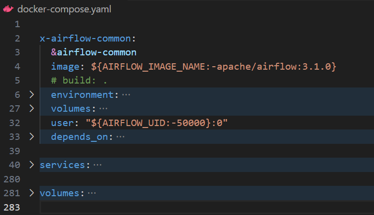
├── docker-compose.yaml
└── README.md

The part-one/ and part-two/ folders contain the complete reference files for our previous tutorials, while the amazon-etl/ folder is the workspace for this project, it contains all the DAGs, helper scripts, and configuration files we’ll build in this lesson. You don’t need to modify anything in the reference folders; they’re just there for review and comparison.

Your starting point is the docker-compose.yaml file, which defines the Airflow services. We’ve already seen how this file manages the Airflow api-server, scheduler, and supporting components.

Next, Airflow expects certain directories to exist before launching. Create them inside the same directory as your docker-compose.yaml file:

mkdir -p ./dags ./logs ./plugins ./config

Now, add a .env file in the same directory with the following line:

AIRFLOW_UID=50000

This ensures consistent file ownership between your host system and Docker containers.

For Linux users, you can generate this automatically with:

echo -e "AIRFLOW_UID=$(id -u)" > .env

Finally, initialize your Airflow metadata database:

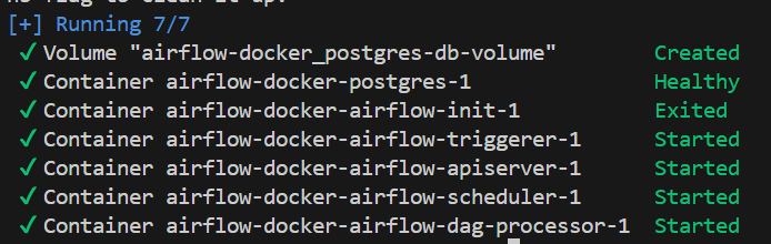
docker compose up airflow-init

Make sure your Docker Desktop is already running before executing the command. Once initialization completes, bring up your Airflow environment:

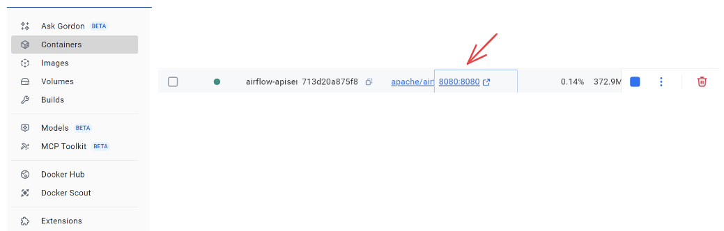
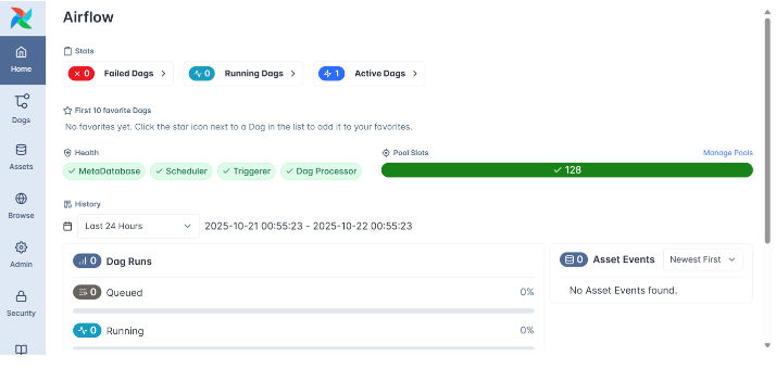
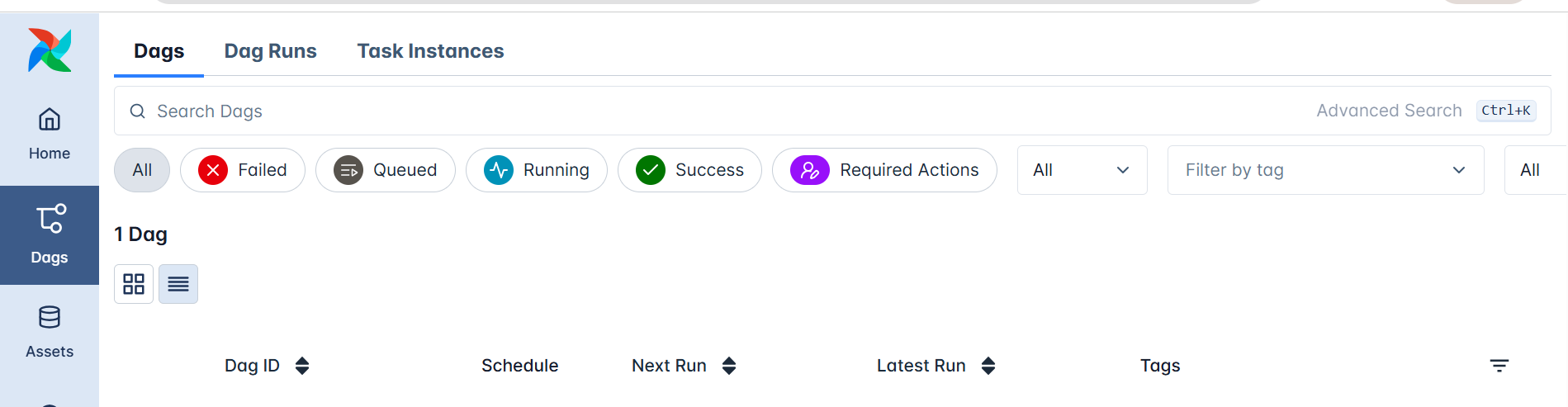
docker compose up -d

If everything is set up correctly, you’ll see all Airflow containers running, including the webserver — which exposes the Airflow UI at http://localhost:8080. Open it in your browser and confirm that your environment is running smoothly by logging in using airflow as the username and airflow as password.

Designing the ETL Pipeline

Now that your environment is ready, it’s time to plan the structure of your ETL workflow before writing any code. Good data engineering practice begins with design, not implementation.

The first step is understanding the data flow, specifically, your source and destination.

In our case:

• The source is Amazon’s public listings for data engineering books.
• The destination is a MySQL database where we’ll store the extracted and transformed data for easy access and analysis.

The workflow will consist of three main stages:

1. Extract – Scrape book information (titles, authors, prices, ratings) from Amazon pages.
2. Transform – Clean and format the raw text into structured, numeric fields using Python and pandas.
3. Load – Insert the processed data into a MySQL table for further use.

At a high level, our data pipeline will look like this:

Amazon Website (Source)
       ↓
   Extract Task
       ↓
   Transform Task
       ↓
   Load Task
       ↓
   MySQL Database (Destination)

To prepare data for loading into MySQL, we’ll need to convert scraped HTML into a tabular structure. The transformation step will include tasks like normalizing currency symbols, parsing ratings into numeric values, and ensuring all records are unique before loading.

When mapped into Airflow, these steps form a Directed Acyclic Graph (DAG) — a visual and logical representation of our workflow. Each box in the DAG represents a task (extract, transform, or load), and the arrows define their dependencies and execution order.

Here’s a conceptual view of the workflow:

[extract_amazon_books] → [transform_amazon_books] → [load_amazon_books]

Finally, we enhance our setup by adding git-sync for automatic DAG updates and GitHub Actions for CI validation, ensuring every change in GitHub reflects instantly in Airflow while your workflows are continuously checked for issues. By combining git-sync, CI checks, and Airflow’s built-in alerting (email or Slack), the entire Amazon ETL pipeline becomes stable, monitored, and much closer to a fully production-like patterns, orchestration system.

Building an ETL Pipeline with Airflow

Setting Up Your DAG File

Let’s start by creating the foundation of our workflow.

Before making changes, make sure to shut down any running containers to avoid conflicts:

docker compose down

Ensure that you disable the Example DAGs and switch to LocalExecutor, as we did in our previous tutorials

Now, open your airflow-docker-tutorial project folder and, inside the dags/ directory, create a new file named:

amazon_etl_dag.py

Every .py file inside this directory becomes a workflow that Airflow automatically detects and manages, no manual registration required. Airflow continuously scans the folder for new DAGs and dynamically loads them.

At the top of your file, import the core libraries needed for this project:

from airflow.decorators import dag, task
from datetime import datetime, timedelta
import pandas as pd
import random
import os
import time
import requests
from bs4 import BeautifulSoup

Let’s quickly review what each import does:

• dag and task come from Airflow’s TaskFlow API, allowing us to define Python functions that become managed tasks, Airflow handles execution, dependencies, and retries automatically.
• datetime and timedelta handle scheduling logic, such as when the DAG should start and how often it should run.
• pandas, random, BeautifulSoup , requests , and os are standard Python libraries we’ll use to process and manage our data within the ETL steps.

This minimal setup is all you need to start orchestrating real-world data workflows.

Defining the DAG Structure

With the imports ready, let’s define the core of our workflow, the DAG configuration.

This determines when, how often, and under what conditions your pipeline runs.

default_args = {
    "owner": "Data Engineering Team",
    "retries": 3,
    "retry_delay": timedelta(minutes=2),
}

@dag(
    dag_id="amazon_books_etl_pipeline",
    description="Automated ETL pipeline to fetch and load Amazon Data Engineering book data into MySQL",
    schedule="@daily",
    start_date=datetime(2025, 11, 13),
    catchup=False,
    default_args=default_args,
    tags=["amazon", "etl", "airflow"],
)
def amazon_books_etl():
    ...

dag = amazon_books_etl()

Let’s break down what’s happening here:

• default_args define reusable settings for all tasks, in this case, Airflow will automatically retry any failed task up to three times, with a two-minute delay between attempts. This is especially useful since our workflow depends on live web requests to Amazon, which can occasionally fail due to rate limits or connectivity issues.
• The @dag decorator marks this function as an Airflow DAG. Everything inside amazon_books_etl() will form part of one cohesive workflow.
• schedule="@daily" ensures our DAG runs once every 24 hours, keeping the dataset fresh.
• start_date defines when Airflow starts scheduling runs.
• catchup=False prevents Airflow from trying to backfill missed runs.
• tags categorize the DAG in the Airflow UI for easier filtering.

Finally, the line:

dag = amazon_books_etl()

instantiates the workflow, making it visible and schedulable within Airflow.

Data Extraction with Airflow

With our DAG structure in place, the first step in our ETL pipeline is data extraction — pulling book data directly from Amazon’s live listings.

• Note that this is for educational purposes: Amazon frequently updates its page structure and uses anti-bot protections, which can break scrapers without warning. In a real production project, we’d rely on official APIs or other stable data sources instead, since they provide consistent data across runs and keep long-term maintenance low.

When you search for something like “data engineering books” on Amazon, the search results page displays listings inside structured HTML containers such as:

<div data-component-type="s-impression-counter">

Each of these containers holds nested elements for the book title, author, price, and rating—information we can reliably parse using BeautifulSoup.

For example, when inspecting any of the listed books, we see a consistent HTML structure that guides how our scraper should behave:

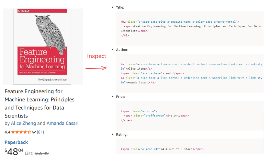
Because Amazon paginates its results, our extraction logic systematically iterates through the first 10 pages, returning approximately 30 to 50 books. We intentionally limit the extraction to this number to keep the workload manageable while still capturing the most relevant items.

This approach ensures we gather the most visible and actively featured books—those trending or recently updated—rather than scraping random or deeply buried results. By looping through these pages, we create a dataset that is both fresh and representative, striking the right balance between completeness and efficiency.

Even though Amazon updates its listings frequently, our Airflow DAG runs every 24 hours, ensuring the extracted data always reflects the latest marketplace activity.

Here’s the Python logic behind the extraction step:

@task
def get_amazon_data_books(num_books=50, max_pages=10, ti=None):
    """
    Extracts Amazon Data Engineering book details such as Title, Author, Price, and Rating. Saves the raw extracted data locally and pushes it to XCom for downstream tasks.
    """
    headers = {
        "Referer": 'https://www.amazon.com/',
        "Sec-Ch-Ua": "Not_A Brand",
        "Sec-Ch-Ua-Mobile": "?0",
        "Sec-Ch-Ua-Platform": "macOS",
        'User-agent': 'Mozilla/5.0 (Macintosh; Intel Mac OS X 10_15_7) AppleWebKit/537.36 (KHTML, like Gecko) Chrome/107.0.0.0 Safari/537.36'
    }

    base_url = "https://www.amazon.com/s?k=data+engineering+books"
    books, seen_titles = [], set()
    page = 1  # start with page 1

    while page <= max_pages and len(books) < num_books:
        url = f"{base_url}&page={page}"

        try:
            response = requests.get(url, headers=headers, timeout=15)
        except requests.RequestException as e:
            print(f" Request failed: {e}")
            break

        if response.status_code != 200:
            print(f"Failed to retrieve page {page} (status {response.status_code})")
            break

        soup = BeautifulSoup(response.text, "html.parser")
        book_containers = soup.find_all("div", {"data-component-type": "s-impression-counter"})

        for book in book_containers:
            title_tag = book.select_one("h2 span")
            author_tag = book.select_one("a.a-size-base.a-link-normal")
            price_tag = book.select_one("span.a-price > span.a-offscreen")
            rating_tag = book.select_one("span.a-icon-alt")

            if title_tag and price_tag:
                title = title_tag.text.strip()
                if title not in seen_titles:
                    seen_titles.add(title)
                    books.append({
                        "Title": title,
                        "Author": author_tag.text.strip() if author_tag else "N/A",
                        "Price": price_tag.text.strip(),
                        "Rating": rating_tag.text.strip() if rating_tag else "N/A"
                    })
        if len(books) >= num_books:
            break

        page += 1
        time.sleep(random.uniform(1.5, 3.0))

    # Convert to DataFrame
    df = pd.DataFrame(books)
    df.drop_duplicates(subset="Title", inplace=True)

    # Create directory for raw data.
        # Note: This works here because everything runs in one container.
        # In real deployments, you'd use shared storage (e.g., S3/GCS) instead.
    os.makedirs("/opt/airflow/tmp", exist_ok=True)
    raw_path = "/opt/airflow/tmp/amazon_books_raw.csv"

    # Save the extracted dataset
    df.to_csv(raw_path, index=False)
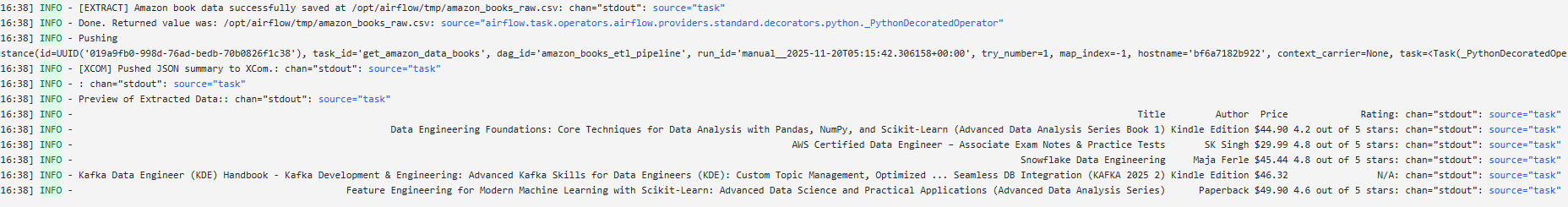
    print(f"[EXTRACT] Amazon book data successfully saved at {raw_path}")

    # Push DataFrame path to XCom
    import json

    summary = {
        "rows": len(df),
        "columns": list(df.columns),
        "sample": df.head(3).to_dict('records'),
    }

    # Clean up non-breaking spaces and format neatly
    formatted_summary = json.dumps(summary, indent=2, ensure_ascii=False).replace('\xa0', ' ')

    if ti:
        ti.xcom_push(key='df_summary', value= formatted_summary)
        print("[XCOM] Pushed JSON summary to XCom.")

    # Optional preview
    print("\nPreview of Extracted Data:")
    print(df.head(5).to_string(index=False))

    return raw_path

This approach makes your pipeline deterministic and meaningful; it doesn’t rely on arbitrary randomness but on a fixed, observable window of recent and visible listings.

You can run this one task and view the logs.

By calling this function, within our def amazon_books_etl() function, we are actually creating a task, and Airflow will consider this as one task:

def amazon_books_etl():
    ---
    # Task dependencies 
    raw_file = get_amazon_data_books()

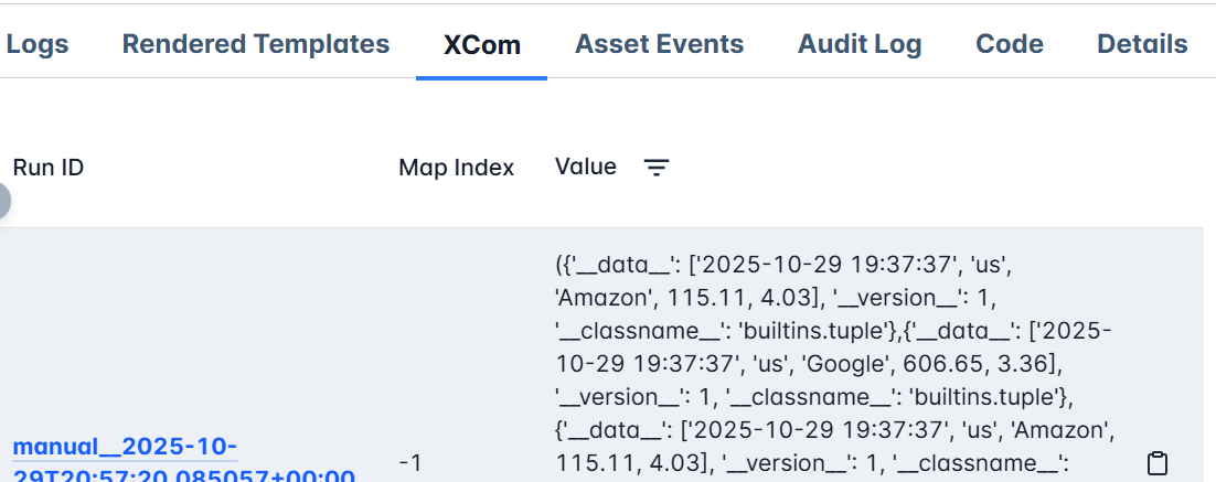
dag = amazon_books_etl()

You should also notice that we are passing a few pieces of information related to our extracted data to XCOM. These include the total length of our dataframe, the total number of columns, and also the first three rows. This will help us understand the transformation(including cleaning) we need for our data.

Data Transformation with Airflow

Once our raw Amazon book data is extracted and stored, the next step is data transformation — converting the messy, unstructured output into a clean, analysis-ready format.

If we inspect the sample data passed through XCom, it looks something like this:

{
  "rows": 42,
  "sample": [
    {
      "Title": "Data Engineering Foundations: Core Techniques for Data Analysis with Pandas, NumPy, and Scikit-Learn (Advanced Data Analysis Series Book 1)",
      "Author": "Kindle Edition",
      "Price": "$44.90",
      "Rating": "4.2 out of 5 stars"
    }
  ],
  "columns": ["Title", "Author", "Price", "Rating"]
}

We can already notice a few data quality issues:

• The Price column includes the dollar sign ($) — we’ll remove it and convert prices to numeric values.
• The Rating column contains text like "4.2 out of 5 stars" — we’ll extract just the numeric part (4.2).
• The Price column name isn’t very clear — we’ll rename it to Price($) for consistency.

Here’s the updated transformation task:

@task
def transform_amazon_books(raw_file: str):
    """
    Standardizes the extracted Amazon book dataset for analysis.
    - Converts price strings (e.g., '$45.99') into numeric values
    - Extracts numeric ratings (e.g., '4.2' from '4.2 out of 5 stars')
    - Renames 'Price' to 'Price($)'
    - Handles missing or unexpected field formats safely
    - Performs light validation after numeric conversion
    """
    if not os.path.exists(raw_file):
        raise FileNotFoundError(f" Raw file not found: {raw_file}")

    df = pd.read_csv(raw_file)
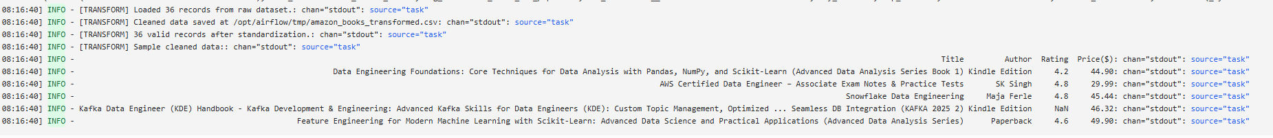
    print(f"[TRANSFORM] Loaded {len(df)} records from raw dataset.")

    # --- Price cleaning (defensive) ---
    if "Price" in df.columns:
        df["Price($)"] = (
            df["Price"]
            .astype(str)                                   # prevents .str on NaN
            .str.replace("$", "", regex=False)
            .str.replace(",", "", regex=False)
            .str.extract(r"(\d+\.?\d*)")[0]                # safely extract numbers
        )
        df["Price($)"] = pd.to_numeric(df["Price($)"], errors="coerce")
    else:
        print("[TRANSFORM] Missing 'Price' column — filling with None.")
        df["Price($)"] = None

    # --- Rating cleaning (defensive) ---
    if "Rating" in df.columns:
        df["Rating"] = (
            df["Rating"]
            .astype(str)
            .str.extract(r"(\d+\.?\d*)")[0]
        )
        df["Rating"] = pd.to_numeric(df["Rating"], errors="coerce")
    else:
        print("[TRANSFORM] Missing 'Rating' column — filling with None.")
        df["Rating"] = None

    # --- Validation: drop rows where BOTH fields failed (optional) ---
    df.dropna(subset=["Price($)", "Rating"], how="all", inplace=True)

    # --- Drop original Price column (if present) ---
    if "Price" in df.columns:
        df.drop(columns=["Price"], inplace=True)

    # --- Save cleaned dataset ---
    transformed_path = raw_file.replace("raw", "transformed")
    df.to_csv(transformed_path, index=False)

    print(f"[TRANSFORM] Cleaned data saved at {transformed_path}")
    print(f"[TRANSFORM] {len(df)} valid records after standardization.")
    print(f"[TRANSFORM] Sample cleaned data:\n{df.head(5).to_string(index=False)}")

    return transformed_path

This transformation ensures that by the time our data reaches the loading stage (MySQL), it’s tidy, consistent, and ready for querying, for instance, to quickly find the highest-rated or most affordable data engineering books.

• Note: Although we’re working with real Amazon data, this transformation logic is intentionally simplified for the purposes of the tutorial. Amazon’s page structure can change, and real-world pipelines typically include more robust safeguards, such as retries, stronger validation rules, fallback parsing strategies, and alerting, so that temporary layout changes or missing fields don’t break the entire workflow. The defensive checks added here help keep the DAG stable, but a production deployment would apply additional hardening to handle a broader range of real-world variations

Data Loading with Airflow

The final step in our ETL pipeline is data loading, moving our transformed dataset into a structured database where it can be queried, analyzed, and visualized.

At this stage, we’ve already extracted live book listings from Amazon and transformed them into clean, numeric-friendly records. Now we’ll store this data in a MySQL database, ensuring that every 24 hours our dataset refreshes with the latest available titles, authors, prices, and ratings.

We’ll use a local MySQL instance for simplicity, but the same logic applies to cloud-hosted databases like Amazon RDS, Google Cloud SQL, or Azure MySQL.

Before proceeding, make sure MySQL is installed and running locally, with a database and user configured as:

CREATE DATABASE airflow_db;
CREATE USER 'airflow'@'%' IDENTIFIED BY 'airflow';
GRANT ALL PRIVILEGES ON airflow_db.* TO 'airflow'@'%';
FLUSH PRIVILEGES;

When running Airflow in Docker and MySQL locally on Linux, Docker containers can’t automatically access localhost.

To fix this, you need to make your local machine reachable from inside Docker.

Open your docker-compose.yaml file and add the following line under the x-airflow-common service definition:

extra_hosts:
  - "host.docker.internal:host-gateway"

Once configured, we can define our load task:

@task
def load_to_mysql(transformed_file: str):
    """
    Loads the transformed Amazon book dataset into a MySQL table for analysis.
    Uses a truncate-and-load pattern to keep the table idempotent.
    """
    import mysql.connector
    import os
    import numpy as np

    # Note:
    # For production-ready projects, database credentials should never be hard-coded.
    # Airflow provides a built-in Connection system and can also integrate with
    # secret backends (AWS Secrets Manager, Vault, etc.).
    #
    # Example:
    #     hook = MySqlHook(mysql_conn_id="my_mysql_conn")
    #     conn = hook.get_conn()
    #
    # For this demo, we keep a simple local config:
    db_config = {
        "host": "host.docker.internal",
        "user": "airflow",
        "password": "airflow",
        "database": "airflow_db",
        "port": 3306
    }

    df = pd.read_csv(transformed_file)
    table_name = "amazon_books_data"

    # Replace NaN with None (important for MySQL compatibility)
    df = df.replace({np.nan: None})

    conn = mysql.connector.connect(**db_config)
    cursor = conn.cursor()

    # Create table if it does not exist
    cursor.execute(f"""
        CREATE TABLE IF NOT EXISTS {table_name} (
            Title VARCHAR(512),
            Author VARCHAR(255),
            `Price($)` DECIMAL(10,2),
            Rating DECIMAL(4,2)
        );
    """)

    # Truncate table for idempotency
    cursor.execute(f"TRUNCATE TABLE {table_name};")

    # Insert rows
    insert_query = f"""
        INSERT INTO {table_name} (Title, Author, `Price($)`, Rating)
        VALUES (%s, %s, %s, %s)
    """

    for _, row in df.iterrows():
        try:
            cursor.execute(
                insert_query,
                (row["Title"], row["Author"], row["Price($)"], row["Rating"])
            )
        except Exception as e:
            # For demo purposes we simply skip bad rows.
            # In real pipelines, you'd log or send them to a dead-letter table.
            print(f"[LOAD] Skipped corrupted row due to error: {e}")

    conn.commit()
    conn.close()

    print(f"[LOAD] Table '{table_name}' refreshed with {len(df)} rows.")

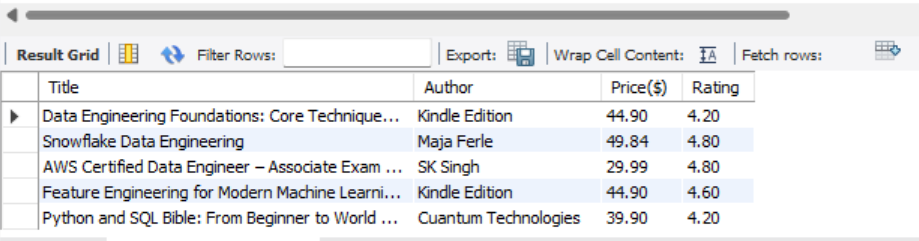
This task reads the cleaned dataset and inserts it into a table named amazon_books_data inside your airflow_db database.

You will also notice that, in the code above that we use a TRUNCATE statement before inserting new rows. This turns the loading step into a full-refresh pattern, making the task idempotent. In other words, running the DAG multiple times produces the same final table instead of accumulating duplicate snapshots from previous days. This is ideal for scraped datasets like Amazon listings, where we want each day’s table to represent only the latest available snapshot.

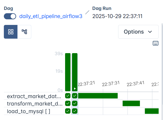
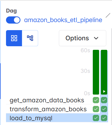
At this stage, your workflow is fully defined and properly instantiated in Airflow, with each task connected in the correct order to form a complete ETL pipeline. Your DAG structure should now look like this:

def amazon_books_etl():
    # Task dependencies
    raw_file = get_amazon_data_books()
    transformed_file = transform_amazon_books(raw_file)
    load_to_mysql(transformed_file)

dag = amazon_books_etl()

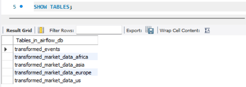
After your DAG runs (use docker compose up -d), you can verify the results inside MySQL:

USE airflow_db;
SHOW TABLES;
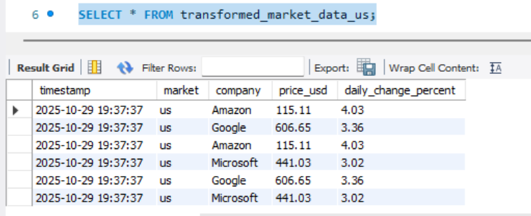
SELECT * FROM amazon_books_data LIMIT 5;

Your table should now contain the latest snapshot of data engineering books, automatically updated daily through Airflow’s scheduling system.

If you'd like, I can also show the Airflow Connection UI configuration example or an example using MySqlHook directly instead of mysql.connector.

Adding Git Sync, CI, and Alerts

At this point, you’ve successfully extracted, transformed, and loaded your data. However, your DAGs are still stored locally on your computer, which makes it difficult for collaborators to contribute and puts your entire workflow at risk if your machine fails or gets corrupted.

In this final section, we’ll introduce a few production-like patterns, version control, automated DAG syncing, basic CI checks, and failure alerts. These don’t make the project fully production-ready, but they represent the core practices most data engineers start with when moving beyond local development. The goal here is to show the essential workflow: storing DAGs in Git, syncing them automatically, validating updates before deployment, and receiving notifications when something breaks.

(For a more detailed explanation of the Git Sync setup shown below, you can read the extended breakdown here.)

To begin, create a public or private repository named airflow_dags (e.g., https://github.com/<your-username>/airflow_dags).

Then, in your project root (airflow-docker), initialize Git and push your local dags/ directory:

git init
git remote add origin https://github.com/<your-username>/airflow_dags.git
git add dags/
git commit -m "Add Airflow ETL pipeline DAGs"
git branch -M main
git push -u origin main

Once complete, your DAGs live safely in GitHub, ready for syncing.

1. Automating Dags with Git Sync

Rather than manually copying DAG files into your Airflow container, we can automate this using git-sync. This lightweight sidecar container continuously clones your GitHub repository into a shared volume.

Each time you push new DAG updates to GitHub, git-sync automatically pulls them into your Airflow environment, no rebuilds, no restarts. This ensures every environment always runs the latest, version-controlled workflow.

As we saw previously, we need to add a new git-sync service to our docker-compose.yaml and create a shared volume called airflow-dags-volume (this can be any name, just make it consistent) that both git-sync and Airflow will use.

services:
  git-sync:
    image: registry.k8s.io/git-sync/git-sync:v4.1.0
    user: "0:0"    # run as root so it can create /dags/git-sync
    restart: always
    environment:
      GITSYNC_REPO: "https://github.com/<your-username>/airflow-dags.git"
      GITSYNC_BRANCH: "main"           # use BRANCH not REF
      GITSYNC_PERIOD: "30s"
      GITSYNC_DEPTH: "1"
      GITSYNC_ROOT: "/dags/git-sync"
      GITSYNC_DEST: "repo"
      GITSYNC_LINK: "current"
      GITSYNC_ONE_TIME: "false"
      GITSYNC_ADD_USER: "true"
      GITSYNC_CHANGE_PERMISSIONS: "1"
      GITSYNC_STALE_WORKTREE_TIMEOUT: "24h"
    volumes:
      - airflow-dags-volume:/dags
    healthcheck:
      test: ["CMD-SHELL", "test -L /dags/git-sync/current && test -d /dags/git-sync/current/dags && [ \"$(ls -A /dags/git-sync/current/dags 2>/dev/null)\" ]"]
      interval: 10s
      timeout: 3s
      retries: 10
      start_period: 10s

volumes:
  airflow-dags-volume:

We then replace the original DAGs mount line in the volumes section(- ${AIRFLOW_PROJ_DIR:-.}/dags:/opt/airflow/dags) with - airflow-dags-volume:/opt/airflow/dags so Airflow reads DAGs directly from the synchronized Git volume.

We also set AIRFLOW__CORE__DAGS_FOLDER to /opt/airflow/dags/git-sync/current/dags so Airflow always points to the latest synced repository.

Finally, each Airflow service (airflow-apiserver, airflow-triggerer, airflow-dag-processor, and airflow-scheduler) is updated with a depends_on condition to ensure they only start after git-sync has successfully cloned the DAGs:

git-sync:
        condition: service_healthy

2. Adding Continuous Integration (CI) with GitHub Actions

To avoid deploying broken DAGs, we can add a lightweight GitHub Actions pipeline that validates DAG syntax before merging into the main branch.

Create a file in your repository:

.github/workflows/validate-dags.yml

name: Validate Airflow DAGs

on:
  push:
    branches: [ main ]
    paths:
      - 'dags/**'

jobs:
  validate:
    runs-on: ubuntu-latest
    steps:
      - uses: actions/checkout@v4
      - uses: actions/setup-python@v5
        with:
          python-version: '3.11'
      # Install all required packages for your DAG imports
      # (instead of only installing Apache Airflow)
      - name: Install dependencies
        run: |
          pip install -r requirements.txt
        # Validate that all DAGs parse correctly
      # This imports every DAG file; if any import fails, CI fails.
      - name: Validate DAGs
        run: |
          echo "Validating DAG syntax..."
          airflow dags list || exit 1

This workflow automatically runs when new DAGs are pushed, ensuring they parse correctly before reaching Airflow.

3. Setting Up Alerts for Failures

Finally, for real-time visibility, Airflow provides alerting mechanisms that can notify you of any failed tasks via email or Slack.

Add this configuration under your DAG’s default_args:

default_args = {
    "owner": "Data Engineering Team",
    "email": ["[email protected]"],
    "email_on_failure": True,
    "retries": 2,
    "retry_delay": timedelta(minutes=5),
}

If an extraction fails (for instance, Amazon changes its HTML structure or MySQL goes offline), Airflow automatically sends an alert with the error log and task details.

Summary and Up Next

In this tutorial, you built a complete, real-world ETL pipeline in Apache Airflow by moving beyond simulated workflows and extracting live book data from Amazon. You designed a production-style workflow that scrapes, cleans, and loads Amazon listings into MySQL, while organizing your code using Airflow’s TaskFlow API for clarity, modularity, and reliability.

You then strengthened your setup by integrating Git-based DAG management with git-sync, adding GitHub Actions CI to automatically validate workflows, and enabling alerting so failures are detected and surfaced immediately.

Together, these improvements transformed your project into a version-controlled, automated orchestration system that mirrors real production environments and prepares you for cloud deployment.

As a next step, you can expand this workflow by exploring other Amazon categories or by applying the same scraping and ETL techniques to entirely different websites, such as OpenWeather for weather insights or Indeed for job listings. This will broaden your data engineering experience with new, real-world data sources. Running Airflow in the cloud is also an important milestone; this tutorial will help you further deepen your understanding of cloud-based Airflow deployments.

In the previous tutorial, we set up Apache Airflow inside Docker, explored its architecture, and built our first real DAG using the TaskFlow API. We simulated an ETL process with two stages — Extract and Transform, demonstrating how Airflow manages dependencies, task retries, and dynamic parallel execution through Dynamic Task Mapping. By the end, we had a functional, scalable workflow capable of processing multiple datasets in parallel, a key building block for modern data pipelines.

In this tutorial, we’ll build on what you created earlier and take a significant step toward production-style orchestration. You’ll complete the ETL lifecycle by adding the Load stage and connecting Airflow to a local MySQL database. This will allow you to load transformed data directly from your pipeline and manage database connections securely using Airflow’s Connections and Environment Variables.

Beyond data loading, you’ll integrate Git and Git Sync into your Airflow environment to enable version control, collaboration, and continuous deployment of DAGs. These practices mirror how data engineering teams manage Airflow projects in real-world settings, promoting consistency, reliability, and scalability, while still keeping the focus on learning and experimentation.

By the end of this part, your Airflow setup will move beyond a simple sandbox and start resembling a production-aligned environment. You’ll have a complete ETL pipeline, from extraction and transformation to loading and automation, and a clear understanding of how professional teams structure and manage their workflows.

Working with MYSQL in Airflow

In the previous section, we built a fully functional Airflow pipeline that dynamically extracted and transformed market data from multiple regions , us, europe, asia, and africa. Each branch of our DAG handled its own extract and transform tasks independently, creating separate CSV files for each region under /opt/airflow/tmp. This setup mimics a real-world data engineering workflow where regional datasets are processed in parallel before being stored or analyzed further.

Now that our transformed datasets are generated, the next logical step is to load them into a database, a critical phase in any ETL pipeline. This not only centralizes your processed data but also allows for downstream analysis, reporting, and integration with BI tools like Power BI or Looker.

While production pipelines often write to cloud-managed databases such as Amazon RDS, Google Cloud SQL, or Azure Database for MySQL, we’ll keep things local and simple by using a MySQL instance on your machine. This approach allows you to test and validate your Airflow workflows without relying on external cloud resources or credentials. The same logic, however, can later be applied seamlessly to remote or cloud-hosted databases.

Prerequisite: Install and Set Up MySQL Locally

Before adding the Load step to our DAG, ensure that MySQL is installed and running on your machine.

Install MySQL

• Windows/macOS: Download and install MySQL Community Server.

• Linux (Ubuntu):

  sudo apt update
  sudo apt install mysql-server -y
  sudo systemctl start mysql
  

• Verify installation by running:

mysql -u root -p

Create a Database and User for Airflow

Inside your MySQL terminal or MySQL Workbench, run the following commands:

CREATE DATABASE IF NOT EXISTS airflow_db;
CREATE USER IF NOT EXISTS 'airflow'@'%' IDENTIFIED BY 'airflow';
GRANT ALL PRIVILEGES ON airflow_db.* TO 'airflow'@'%';
FLUSH PRIVILEGES;

This creates a simple local database called airflow_db and a user airflow with full access, perfect for development and testing.

Network Configuration for Linux Users

When running Airflow in Docker and MySQL locally on Linux, Docker containers can’t automatically access localhost.

To fix this, you need to make your local machine reachable from inside Docker.

Open your docker-compose.yaml file and add the following line under the x-airflow-common service definition:

extra_hosts:
  - "host.docker.internal:host-gateway"

This line creates a bridge that allows Airflow containers to communicate with your local MySQL instance using the hostname host.docker.internal.

Switching to LocalExecutor

In part one of this tutorial, we worked with CeleryExecutor to run our Airflow. By default, the Docker Compose file uses CeleryExecutor, which requires additional components such as Redis, Celery workers, and the Flower dashboard for distributed task execution.

Since we’re running Airflow to make it production-ready, we can simplify things by using LocalExecutor, which runs tasks in parallel on a single machine, eliminating the need for an external queue or worker system.

Find this line in your docker-compose.yaml:

AIRFLOW__CORE__EXECUTOR: CeleryExecutor 

Change it to:

AIRFLOW__CORE__EXECUTOR: LocalExecutor

Removing Unnecessary Services

Because we’re no longer using Celery, we can safely remove related components from the configuration. These include Redis, airflow-worker, and Flower.

You can search for the following sections and delete them:

• The entire redis service block.
• The airflow-worker service (Celery’s worker).
• The flower service (Celery monitoring dashboard).
• Any AIRFLOW__CELERY__... lines inside environment blocks.

Extending the DAG with a Load Step

Now let’s extend our existing DAG to include the Load phase of the ETL process. Already we had extract_market_data() and transform_market_data() created in the first part of this tutorial. This new task will read each transformed CSV file and insert its data into a MySQL table.

Here’s our updated daily_etl_pipeline_airflow3 DAG with the new load_to_mysql() task.
You can also find the complete version of this DAG in the cloned repository([email protected]:dataquestio/tutorials.git), inside the part-two/

folder under airflow-docker-tutorial .

def daily_etl_pipeline():

    @task
    def extract_market_data(market: str):
        ...

    @task
    def transform_market_data(raw_file: str):
        ...

    @task
    def load_to_mysql(transformed_file: str):
        """Load the transformed CSV data into a MySQL table."""
        import mysql.connector
        import os

        db_config = {
            "host": "host.docker.internal",  # enables Docker-to-local communication
            "user": "airflow",
            "password": "airflow",
            "database": "airflow_db",
            "port": 3306
        }

        df = pd.read_csv(transformed_file)

        # Derive the table name dynamically based on region
        table_name = f"transformed_market_data_{os.path.basename(transformed_file).split('_')[-1].replace('.csv', '')}"

        conn = mysql.connector.connect(**db_config)
        cursor = conn.cursor()

        # Create table if it doesn’t exist
        cursor.execute(f"""
            CREATE TABLE IF NOT EXISTS {table_name} (
                timestamp VARCHAR(50),
                market VARCHAR(50),
                company VARCHAR(255),
                price_usd DECIMAL,
                daily_change_percent DECIMAL
            );
        """)

        # Insert records
        for _, row in df.iterrows():
            cursor.execute(
                f"""
                INSERT INTO {table_name} (timestamp, market, company, price_usd, daily_change_percent)
                VALUES (%s, %s, %s, %s, %s)
                """,
                tuple(row)
            )

        conn.commit()
        conn.close()
        print(f"[LOAD] Data successfully loaded into MySQL table: {table_name}")

    # Define markets to process dynamically
    markets = ["us", "europe", "asia", "africa"]

    # Dynamically create and link tasks
    raw_files = extract_market_data.expand(market=markets)
    transformed_files = transform_market_data.expand(raw_file=raw_files)
    load_to_mysql.expand(transformed_file=transformed_files)

dag = daily_etl_pipeline()

When you trigger this DAG, Airflow will automatically create three sequential tasks for each defined region (us, europe, asia, africa):

first extracting market data, then transforming it, and finally loading it into a region-specific MySQL table.

Each branch runs independently, so by the end of a successful run, your local MySQL database (airflow_db) will contain four separate tables, one for each region:

transformed_market_data_us
transformed_market_data_europe
transformed_market_data_asia
transformed_market_data_africa

Each table contains the cleaned and sorted dataset for its region, including company names, prices, and daily percentage changes.

Once your containers are running, open MySQL (via terminal or MySQL Workbench) and run:

SHOW TABLES;

You should see all four tables listed. Then, to inspect one of them, for example us, run:

SELECT * FROM transformed_market_data_us;

From above, we can see the dataset that Airflow extracted, transformed, and loaded for the U.S. market, confirming your pipeline has now completed all three stages of ETL: Extract → Transform → Load.

This integration demonstrates Airflow’s ability to manage data flow across multiple sources and databases seamlessly, a key capability in modern data engineering pipelines.

Absolutely, here’s the updated subsection with your requested note added in the right place.

It keeps the professional teaching tone and gently reminds learners that these connection values must match the local MySQL setup they created earlier.

Previewing the Loaded Data in Airflow

By now, you’ve confirmed that your transformed datasets are successfully loaded into MySQL, you can view them directly in MySQL Workbench or through a SQL client. But Airflow also provides a convenient way to query and preview this data right from the UI, using Connections and the SQLExecuteQueryOperator.

Connections in Airflow store the credentials and parameters needed to connect to external systems such as databases, APIs, or cloud services. Instead of hardcoding passwords or host details in your DAGs, you define a connection once in the Web UI and reference it securely using its conn_id.

To set this up:

1. Open the Airflow Web UI
2. Navigate to Admin → Connections → + Add a new record
3. Fill in the following details:

Field	Value
Conn Id	local_mysql
Conn Type	MySQL
Host	host.docker.internal
Schema	airflow_db
Login	airflow
Password	airflow
Port	3306

Note: These values must match the credentials you defined earlier when setting up your local MySQL instance.

Specifically, the database airflow_db, user airflow, and password airflow should already exist in your MySQL setup.

The host.docker.internal value ensures that your Airflow containers can communicate with MySQL running on your local machine.

• Also note that when you use docker compose down -v, all volumes, including your Airflow connections, will be deleted. Always remember to re-add the connection afterward.

If your changes are not volume-related, you can safely shut down the containers using docker compose down (without -v), which preserves your existing connections and data.

Click Save to register the connection.

Now, Airflow knows how to connect to your MySQL database whenever a task specifies conn_id="local_mysql".

Let’s create a simple SQL query task to preview the data we just loaded.

    @task
    def extract_market_data(market: str):
        ...

    @task
    def transform_market_data(raw_file: str):
        ...

    @task
    def load_to_mysql(transformed_file: str):
        ...

        from airflow.providers.common.sql.operators.sql import SQLExecuteQueryOperator

        preview_mysql = SQLExecuteQueryOperator(
            task_id="preview_mysql_table",
            conn_id="local_mysql",
            sql="SELECT * FROM transformed_market_data_us LIMIT 5;",
            do_xcom_push=True,  # makes query results viewable in Airflow’s XCom tab
        )
        # Dynamically create and link tasks
    raw_files = extract_market_data.expand(market=markets)
    transformed_files = transform_market_data.expand(raw_file=raw_files)
    load_to_mysql.expand(transformed_file=transformed_files)

dag = daily_etl_pipeline()

Next, link this task to your DAG so that it runs after the loading process, update this line load_to_mysql.expand(transformed_file=transformed_files) to this:

    load_to_mysql.expand(transformed_file=transformed_files) >> preview_mysql

When you trigger the DAG again (always remember to shut down the containers before making changes to your DAGs using docker compose down, and then, once saved, use docker compose up -d), Airflow will:

1. Connect to your MySQL database using the stored connection credentials.
2. Run the SQL query on the specified table.
3. Display the first few rows of your data as a JSON result in the XCom view.

To see it:

• Go to Grid View
• Click on the preview_mysql_table task
• Choose XCom from the top menu

You’ll see your data represented in JSON format, confirming that the integration works, Airflow not only orchestrates the workflow but can also interactively query and visualize your results without leaving the platform.

This makes it easy to verify that your ETL pipeline is functioning correctly end-to-end: extraction, transformation, loading, and now validation, all visible and traceable inside Airflow.

Git-Based DAG Management and CI/CD for Deployment (with git-sync)

At this stage, your local Airflow environment is complete, you’ve built a fully functional ETL pipeline that extracts, transforms, and loads regional market data into MySQL, and even validated results directly from the Airflow UI.

Now it’s time to take the final step toward production readiness: managing your DAGs the way data engineering teams do in real-world systems, through Git-based deployment and continuous integration.

We’ll push our DAGs to a shared GitHub repository called airflow_dags, and connect Airflow to it using the git-sync container, which automatically keeps your DAGs in sync. This allows every team member (or environment) to pull from the same source, the Git repo, without manually copying files into containers.

Why Manage DAGs with Git

Every DAG is just a Python file, and like all code, it deserves version control. Storing DAGs in a Git repository brings the same advantages that software engineers rely on:

• Versioning: track every change and roll back safely.
• Collaboration: multiple developers can work on different workflows without conflict.
• Reproducibility: every environment can pull identical DAGs from a single source.
• Automation: changes sync automatically, eliminating manual uploads.

This structure makes Airflow easier to maintain and scales naturally as your pipelines grow in number and complexity.

Pushing Your DAGs to GitHub

To begin, create a public or private repository named airflow_dags (e.g., https://github.com/<your-username>/airflow_dags).

Then, in your project root (airflow-docker), initialize Git and push your local dags/ directory:

git init
git remote add origin https://github.com/<your-username>/airflow_dags.git
git add dags/
git commit -m "Add Airflow ETL pipeline DAGs"
git branch -M main
git push -u origin main

Once complete, your DAGs live safely in GitHub, ready for syncing.

How git-sync Works

git-sync is a lightweight sidecar container that continuously clones and updates a Git repository into a shared volume.

Once running, it:

• Clones your repository (e.g., https://github.com/<your-username>/airflow_dags.git),
• Pulls updates every 30 seconds by default,
• Exposes the latest DAGs to Airflow automatically, no rebuilds or restarts required.

This is how Airflow stays up to date with your Git repo in real time.

Setting Up git-sync in Docker Compose

In your existing docker-compose.yaml, you already have a list of services that define your Airflow environment, like the api-server, scheduler, triggerer, and dag-processor. Each of these runs in its own container but works together as part of the same orchestration system.

The git-sync container will become another service in this list, just like those, but with a very specific purpose:

• to keep your /dags folder continuously synchronized with your remote GitHub repository.

Instead of copying Python DAG files manually or rebuilding containers every time you make a change, the git-sync service will automatically pull updates from your GitHub repo (in our case, airflow_dags) into a shared volume that all Airflow services can read from.

This ensures that your environment always runs the latest DAGs from GitHub ,without downtime, restarts, or manual synchronization.

Remember in our docker-compose.yaml file, we had this kind of setup:

Now, we’ll extend that structure by introducing git-sync as an additional service within the same services: section and also an addition in the volumes: section(other than postgres-db-volume: we we have to also add airflow-dags-volume: for uniformity accross all containers).

Below is a configuration that works seamlessly with Docker on any OS:

services:
  git-sync:
    image: registry.k8s.io/git-sync/git-sync:v4.1.0
    user: "0:0"    # run as root so it can create /dags/git-sync
    restart: always
    environment:
      GITSYNC_REPO: "https://github.com/<your-username>/airflow-dags.git"
      GITSYNC_BRANCH: "main"           # use BRANCH not REF
      GITSYNC_PERIOD: "30s"
      GITSYNC_DEPTH: "1"
      GITSYNC_ROOT: "/dags/git-sync"
      GITSYNC_DEST: "repo"
      GITSYNC_LINK: "current"
      GITSYNC_ONE_TIME: "false"
      GITSYNC_ADD_USER: "true"
      GITSYNC_CHANGE_PERMISSIONS: "1"
      GITSYNC_STALE_WORKTREE_TIMEOUT: "24h"
    volumes:
      - airflow-dags-volume:/dags
    healthcheck:
      test: ["CMD-SHELL", "test -L /dags/git-sync/current && test -d /dags/git-sync/current/dags && [ \"$(ls -A /dags/git-sync/current/dags 2>/dev/null)\" ]"]
      interval: 10s
      timeout: 3s
      retries: 10
      start_period: 10s

volumes:
  airflow-dags-volume:

In this setup, the git-sync service runs as a lightweight companion container that keeps your Airflow DAGs in sync with your GitHub repository.

The GITSYNC_REPO variable tells it where to pull code from, in this case, your DAG repository (airflow_dags). Make sure you replace <your-username> with your exact GitHub username. The GITSYNC_BRANCH specifies which branch to track, usually main, while GITSYNC_PERIOD defines how often to check for updates. Here, it’s set to every 30 seconds, meaning Airflow will always be within half a minute of your latest Git push.

The synchronization happens inside the directory defined by GITSYNC_ROOT, which becomes /dags/git-sync inside the container. Inside that root, GITSYNC_DEST defines where the repo is cloned (as repo), and GITSYNC_LINK creates a symbolic link called current pointing to the active clone.

This design allows Airflow to always reference a stable, predictable path (/dags/git-sync/current/dags) even as the repository updates in the background, no path changes, no reloads.

A few environment flags ensure stability and portability across systems. For instance, GITSYNC_ADD_USER and GITSYNC_CHANGE_PERMISSIONS make sure the synced files are accessible to Airflow even when permissions differ across Docker environments.

GITSYNC_DEPTH limits the clone to just the latest commit (keeping it lightweight), while GITSYNC_STALE_WORKTREE_TIMEOUT helps clean up old syncs if something goes wrong.

The shared volume, airflow-dags-volume, acts as the bridge between git-sync and Airflow. It stores all synced DAGs in one central location accessible by both containers. The health check at the end ensures that git-sync is functioning, it verifies that the /current/dags directory exists and contains files before Airflow tries to load them.

Finally, the healthcheck section ensures that Airflow doesn’t start until git-sync has successfully cloned your repository. It runs a small shell command that checks three things, whether the symbolic link /dags/git-sync/current exists, whether the dags directory is present inside it, and whether that directory actually contains files. Only when all these conditions pass does Docker mark the git-sync service as healthy. The interval and retry parameters control how often and how long these checks run, ensuring that Airflow’s scheduler, webserver, and other components wait patiently until the DAGs are fully available. This simple step prevents race conditions and guarantees a smooth startup every time.

Together, these settings ensure that your Airflow instance always runs the latest DAGs from GitHub, automatically, securely, and without manual file transfers.

Generally, this configuration does the following:

• Creates a shared volume (airflow-dags-volume) where the DAGs are cloned.
• Mounts it into both git-sync and Airflow services.
• Runs git-sync as root to fix permission issues on Windows.
• Keeps DAGs up to date every 30 seconds.

Adjusting the Airflow Configuration

We’ve now added git-sync as part of our Airflow services, sitting right alongside the api-server, scheduler, triggerer, and dag-processor.

This new service continuously pulls our DAGs from GitHub and stores them inside a shared volume (airflow-dags-volume) that both git-sync and Airflow can access.

However, our Airflow setup still expects to find DAGs through local directory mounts defined under each service (via x-airflow-common), not global named volumes. The default configuration maps these paths as follows:

volumes:
    - ${AIRFLOW_PROJ_DIR:-.}/dags:/opt/airflow/dags
    - ${AIRFLOW_PROJ_DIR:-.}/logs:/opt/airflow/logs
    - ${AIRFLOW_PROJ_DIR:-.}/config:/opt/airflow/config
    - ${AIRFLOW_PROJ_DIR:-.}/plugins:/opt/airflow/plugins

This setup points Airflow to the local dags/ folder in your host machine, but now that we have git-sync, our DAGs will live inside a synchronized Git directory instead.

So we need to update the DAG volume mapping to pull from the new shared Git volume instead of the local one.

Replace the first line(- ${AIRFLOW_PROJ_DIR:-.}/dags:/opt/airflow/dags) under the volumes: section with: - airflow-dags-volume:/opt/airflow/dags

This tells Docker to mount the shared airflow-dags-volume (created by git-sync) into Airflow’s /opt/airflow/dags directory.

That way, any DAGs pulled by git-sync from your GitHub repository will immediately appear inside Airflow’s working environment, without needing to rebuild or copy files.

We also need to explicitly tell Airflow where the synced DAGs live.

In the environment section of your x-airflow-common block, add the following:

AIRFLOW__CORE__DAGS_FOLDER: /opt/airflow/dags/git-sync/current/dags

This line links Airflow directly to the directory created by the git-sync container.

Here’s how it connects:

• Inside the git-sync configuration, we defined:

  GITSYNC_ROOT: "/dags/git-sync"
  GITSYNC_LINK: "current"

  Together, these ensure that the most recent repository clone is always available under /dags/git-sync/current.

• When we mount airflow-dags-volume:/opt/airflow/dags, this path becomes accessible inside the Airflow containers as

  /opt/airflow/dags/git-sync/current/dags.

By setting AIRFLOW__CORE__DAGS_FOLDER to that exact path, Airflow automatically watches the live Git-synced DAG directory for changes, meaning every new commit to your GitHub repo will reflect instantly in the Airflow UI.

Finally, ensure that Airflow waits for git-sync to finish cloning before starting up.

In each Airflow service (airflow-scheduler, airflow-apiserver, dag-processor, and triggerer), depends_on section, add:

depends_on:
  git-sync:
    condition: service_healthy

This guarantees that Airflow only starts once the git-sync container has successfully pulled your repository, preventing race conditions during startup.

Once complete, Airflow will read its DAGs directly from the synchronized Git directory , /opt/airflow/dags/git-sync/current/dags , instead of your local project folder.

This change transforms your setup into a live, Git-driven workflow, where Airflow continuously tracks and loads the latest DAGs from GitHub automatically.

Automating Validation with GitHub Actions

Our Git integration wouldn’t be truly powerful without CI/CD (Continuous Integration and Continuous Deployment).

While git-sync ensures that any change pushed to GitHub automatically reflects in Airflow, that alone can be risky, not every change should make it to production immediately.

Imagine pushing a DAG with a missing import, a syntax error, or a bad dependency.

Airflow might fail to parse it, causing your scheduler or api-server to crash or restart repeatedly. That’s why we need a safety net, a way to automatically check that every DAG in our repository is valid before it ever reaches Airflow.

This is exactly where GitHub Actions comes in.

We can set up a lightweight CI pipeline that validates all DAGs whenever someone pushes to the main branch. If a broken DAG is detected, the pipeline fails, preventing the merge and protecting your Airflow environment from unverified code.

GitHub also provides notifications directly in your repository interface, showing failed workflows and highlighting the cause of the issue.

Inside your airflow_dags repository, create a GitHub Actions workflow file at:

.github/workflows/validate-dags.yml

name: Validate Airflow DAGs

on:
  push:
    branches: [ main ]
    paths:
      - 'dags/**'

jobs:
  validate:
    runs-on: ubuntu-latest
    steps:
      - name: Checkout Repository
        uses: actions/checkout@v4

      - name: Set up Python
        uses: actions/setup-python@v5
        with:
          python-version: '3.11'

      - name: Install Airflow
        run: pip install apache-airflow==3.1.1

      - name: Validate DAGs
        run: |
          echo "Validating DAG syntax..."
          airflow dags list || exit 1

This simple workflow automatically runs every time you push a new commit to the main branch (or modify anything in the dags/ directory).

It installs Apache Airflow in a lightweight test environment, loads all your DAGs, and checks that they parse successfully, no missing imports, syntax issues, or circular dependencies.

If even one DAG fails to load, the validation job will exit with an error, causing the GitHub Actions pipeline to fail.

GitHub then immediately notifies you (and any collaborators) through the repository’s Actions tab, issue alerts, and optional email notifications.

By doing this, you’re adding a crucial layer of protection to your workflow:

• Pre-deployment safety: invalid DAGs never reach your running Airflow instance.
• Automatic feedback: failed DAGs trigger GitHub notifications, allowing you to fix errors early.
• Confidence in deployment: once the pipeline passes, you know every DAG is production-ready.

Together, this CI validation and your git-sync setup create a self-updating, automated Airflow environment that mirrors production deployment practices.

With this final step, your Airflow environment becomes a versioned, automated, and production-ready orchestration system, capable of handling real data pipelines the way modern engineering teams do.

You’ve now completed a full transformation:

from local DAG development to automated, Git-driven deployment, all within Docker, all powered by Apache Airflow.

• Note that, both the git-sync service and the Airflow UI depend on your Docker containers running. As long as your containers are up, git-sync remains active, continuously checking for updates in your GitHub repository and syncing any new DAGs to your Airflow environment.

  Once you stop or shut down the containers (docker compose down), this synchronization pauses. You also won’t be able to access the Airflow Web UI or trigger DAGs until the containers are started again.

  When you restart with docker compose up -d, everything, including git-sync , resumes automatically, picking up the latest changes from GitHub and restoring your full Airflow setup just as you left it.

Summary and Up Next

In this tutorial, you completed the ETL lifecycle in Apache Airflow by adding the Load phase to your In this tutorial, you completed the ETL lifecycle in Apache Airflow by adding the Load phase to your workflow and connecting it to a local MySQL database. You learned how Airflow securely manages external connections, dynamically handles multiple data regions, and enables in-UI data previews through XCom and Connections.

You also took your setup a step closer to production by integrating Git-based DAG management with git-sync, and implementing GitHub Actions CI to validate DAGs automatically before deployment.

Together, these changes transformed your environment into a version-controlled, automated orchestration system that mirrors the structure of production-grade setups, a final step before deploying to the cloud.

In the next tutorial, you’ll move beyond simulated data and build a real-world data pipeline, extracting data from an API, transforming it with Python, and loading it into MySQL. You’ll also add retries, alerts, and monitoring, and deploy the full workflow through CI/CD, achieving a truly end-to-end, production-grade Airflow setup.

In the last tutorial, we explored what workflow orchestration is, why it matters, and how Apache Airflow structures, automates, and monitors complex data pipelines through DAGs, tasks, and the scheduler. We examined how orchestration transforms scattered scripts into a coordinated system that ensures reliability, observability, and scalability across modern data workflows.

In this two-part hands-on tutorial, we move from theory to practice. You’ll run Apache Airflow inside Docker, the most efficient and production-like way to deploy Airflow for development and testing. This containerized approach mirrors how Airflow operates in real-world environments, from on-premises teams to managed services like ECR and Cloud Composer.

In Part One, our focus goes beyond setup. You’ll learn how to work effectively with DAGs inside a Dockerized Airflow environment, writing, testing, visualizing, and managing them through the Web UI. You’ll use the TaskFlow API to build clean, Pythonic workflows and implement dynamic task mapping to run multiple processes in parallel. By the end of this part, you’ll have a fully functional Airflow environment running in Docker and a working DAG that extracts and transforms data automatically, the foundation of modern data engineering pipelines.

In Part Two, we’ll extend that foundation to handle data management and automation workflows. You’ll connect Airflow to a local MySQL database for data loading, manage credentials securely through the Admin panel and environment variables, and integrate Git with Git Sync to enable version control and continuous deployment. You’ll also see how CI/CD pipelines can automate DAG validation and deployment, ensuring your Airflow environment remains consistent and collaborative across development teams.

By the end of the series, you’ll not only understand how Airflow runs inside Docker but also how to design, orchestrate, and manage production-grade data pipelines the way data engineers do in real-world systems.

Why Use Docker for Airflow

While Airflow can be installed locally with pip install apache-airflow, this approach often leads to dependency conflicts, version mismatches, and complicated setups. Airflow depends on multiple services, an API server, scheduler, triggerer, metadata database, and dag-processors, all of which must communicate correctly. Installing and maintaining these manually on your local machine can be tedious and error-prone.

Docker eliminates these issues by packaging everything into lightweight, isolated containers. Each container runs a single Airflow component, but all work together seamlessly through Docker Compose. The result is a clean, reproducible environment that behaves consistently across operating systems.

In short:

• Local installation: works for testing but often breaks due to dependency conflicts or version mismatches.
• Cloud-managed services (like AWS ECS or Cloud Composer): excellent for production but not that much flexible for learning or prototyping.
• Docker setup: combines realism with simplicity, providing the same multi-service environment used in production without the overhead of manual configuration.

Docker setup is ideal for learning and development and closely mirrors production environments, but additional configuration is needed for a full production deployment

Prerequisites

Before you begin, ensure the following are installed and ready on your system:

1. Docker Desktop – Required to build and run Airflow containers.
2. A code editor – Visual Studio Code or similar, for writing and editing DAGs.
3. Python 3.10 or higher – Used for authoring Airflow DAGs and helper scripts.

Running Airflow Using Docker

Now that your environment is ready (Docker is open and running), let’s get Airflow running using Docker Compose.

This tool orchestrates all Airflow services, api-server, scheduler, triggerer, database, and workers — so they start and communicate properly.

Clone the Tutorial Repository

We’ve already prepared the starter files you’ll need for this tutorial on GitHub.

Begin by cloning the repository:

git clone [email protected]:dataquestio/tutorials.git

Then navigate to the Airflow tutorial folder:

cd airflow-docker-tutorial

This is the directory where you’ll be working throughout the tutorial.

Inside, you’ll notice a structure similar to this:

airflow-docker-tutorial/
├── part-one/  
├── part-two/
├── docker-compose.yaml
└── README.md

• The part-one/ and part-two/ folders contain the complete reference files for both tutorials (Part One and Part Two).

  You don’t need to modify anything there, it’s only for comparison or review.

• The docker-compose.yaml file is your starting point and will evolve as the tutorial progresses.

Explore the Docker Compose File

Open the docker-compose.yaml file in your code editor.

This file defines all the Airflow components and how they interact inside Docker.

It includes:

• api-server – Airflow’s web user interface
• Scheduler – Parses and triggers DAGs
• Triggerer – Manages deferrable tasks efficiently
• Metadata database – Tracks DAG runs and task states
• Executors – Execute tasks

Each of these services runs in its own container, but together they form a single working Airflow environment.

You’ll be updating this file as you move through the tutorial to configure, extend, and manage your Airflow setup.

Create Required Folders

Airflow expects certain directories to exist before launching.

Create them inside the same directory as your docker-compose.yaml file:

mkdir -p ./dags ./logs ./plugins ./config

• dags/ – your workflow scripts
• logs/ – task execution logs
• plugins/ – custom hooks and operators
• config/ – optional configuration overrides (this will be auto-populated later when initializing the database)

Configure User Permissions

If you’re using Linux, set a user ID to prevent permission issues when Docker writes files locally:

echo -e "AIRFLOW_UID=$(id -u)" > .env

If you’re using macOS or Windows, manually create a .env file in the same directory with the following content:

AIRFLOW_UID=50000

This ensures consistent file ownership between your host system and the Docker containers.

Initialize the Metadata Database

Airflow keeps track of DAG runs, task states, and configurations in a metadata database.

Initialize it by running:

docker compose up airflow-init

Once initialization completes, you’ll see a message confirming that an admin user has been created with default credentials:

• Username: airflow
• Password: airflow

Start Airflow

Now start all Airflow services in the background:

docker compose up -d

Docker Compose will spin up the scheduler, API server, triggerer, database, and worker containers.

Step 6: Start Airflow

Now launch all the services in the background:

docker compose up -d

Docker Compose will start the scheduler, api-server, triggerer, database, and executor containers.

Make sure the triggerer, dag-processor, scheduler, and api-server are shown as started as above. If that is not the case, rebuild the Docker container, since the build process might have been interrupted. Otherwise, navigate to http://localhost:8080 to access the Airflow UI exposed by the api-server.

You can also access this through your Docker app, by navigating to containers:

Log in using the credentials above to accessh the Airflow Web UI.

• If the UI fails to load or some containers keep restarting, increase Docker’s memory allocation to at least 4 GB (8 GB recommended) in Docker Desktop → Settings → Resources.

Configuring the Airflow Project

Once Airflow is running and you visit http://localhost:8080, you’ll be seee Airflow Web UI.

This is the command center for your workflows, where you can visualize DAGs, monitor task runs, and manage system configurations. When you navigate to Dags, you’ll see a dashboard that lists several example DAGs provided by the Airflow team. These are sample workflows meant to demonstrate different operators, sensors, and features.

However, for this tutorial, we’ll build our own clean environment, so we’ll remove these example DAGs and customize our setup to suit our project.

Before doing that, though, it’s important to understand the docker-compose.yaml file, since this is where your Airflow environment is actually defined.

Understanding the docker-compose.yaml File

The docker-compose.yaml file tells Docker how to build, connect, and run all the Airflow components as containers.

If you open it, you’ll see multiple sections that look like this:

Let’s break this down briefly:

• x-airflow-common – This is the shared configuration block that all Airflow containers inherit from. It defines the base Docker image (apache/airflow:3.1.0), key environment variables, and mounted volumes for DAGs, logs, and plugins. It also specifies user permissions to ensure that files created inside the containers are accessible from your host machine. The depends_on lists dependencies such as the PostgreSQL database used to store Airflow metadata. In short, this section sets up the common foundation for every container in your environment.
• services – This section defines the actual Airflow components that make up your environment. Each service, such as the api-server, scheduler, triggerer, dag-processor , and metadata database, runs as a separate container but uses the shared configuration from x-airflow-common. Together, they form a complete Airflow deployment where each container plays a specific role.
• volumes - this section sets up persistent storage for containers. Airflow uses it by default for the Postgres database, keeping your DAGs, logs, and configurations saved across runs. In part 2, we’ll expand it to include Git integration.

Each of these sections works together to create a unified Airflow environment that’s easy to configure, extend, or simplify as needed.

Understanding these parts now will make the next steps - cleaning, customizing, and managing your Airflow setup - much clearer.

Resetting the Environment Before Making Changes

Before editing anything inside the docker-compose.yaml, it’s crucial to shut down your containers cleanly to avoid conflicts.

Run: docker compose down -v

Here’s what this does:

• docker compose down stops and removes all containers.

• The v flag removes volumes, which clears stored metadata, logs, and configurations.

  This ensures that you start with a completely fresh environment the next time you launch Airflow — which can be helpful when your environment becomes misconfigured or broken. However, you shouldn’t do this routinely after every DAG or configuration change, as it will also remove your saved Connections, Variables, and other stateful data. In most cases, you can simply run docker compose down instead to stop the containers without wiping the environment.

Disabling Example DAGs

By default, Airflow loads several example DAGs to help new users explore its features. For our purposes, we want a clean workspace that only shows our own DAGs.

1. Open the docker-compose.yaml file in your code editor.
2. Locate the environment section under x-airflow-common and find this line: AIRFLOW__CORE__LOAD_EXAMPLES: 'true' . Change 'true' to 'false': AIRFLOW__CORE__LOAD_EXAMPLES: 'false'

This setting tells Airflow not to load any of the example workflows when it starts.

Once you’ve made the changes:

1. Save your docker-compose.yaml file.
2. Rebuild and start your Airflow environment again: docker compose up -d
3. Wait a few moments, then visit http://localhost:8080 again.

This time, when you log in, you’ll notice the example DAGs are gone, leaving you with a clean workspace ready for your own workflows.

Let’s now build our first DAG.

Working with DAGs in Airflow

Now that your Airflow environment is clean and running, it’s time to create **** our first real workflow.

This is where you begin writing DAGs (Directed Acyclic Graphs), which sit at the very heart of how Airflow operates.

A DAG is more than just a piece of code, it’s a visual and logical representation of your workflow, showing how tasks connect, when they run, and in what order.

Each task in a DAG represents a distinct step in your process, such as pulling data, cleaning it, transforming it, or loading it into a database. In this tutorial we will create tasks that extract and transform data. We will the see the loading process in part two, and how airflow intergrates to git.

Airflow ensures these tasks execute in the correct order without looping back on themselves (that’s what acyclic means).

Setting Up Your DAG File

Let’s start by creating the foundation of our workflow( make sure to shut down the running containers by using docker compose down -v)

Open your airflow-docker project folder and, inside the dags/ directory, create a new file named:

our_first_dag.py

Every .py file you place in this folder becomes a workflow that Airflow can recognize and manage automatically.

You don’t need to manually register anything, Airflow continuously scans this directory and loads any valid DAGs it finds.

At the top of our file, let’s import the core libraries we need for our project:

from airflow.decorators import dag, task
from datetime import datetime, timedelta
import pandas as pd
import random
import os

Let’s pause to understand what each of these imports does and why they matter:

• dag and task come from Airflow’s TaskFlow API.

  These decorators turn plain Python functions into Airflow-managed tasks, giving you cleaner, more intuitive code while Airflow handles orchestration behind the scenes.

• datetime and timedelta handle scheduling logic.

  They help define when your DAG starts and how frequently it runs.

• pandas, random, and os are standard Python libraries we’ll use to simulate a simple ETL process, generating, transforming, and saving data locally.

This setup might seem minimal, but it’s everything you need to start orchestrating real tasks.

Defining the DAG Structure

With our imports ready, the next step is to define the skeleton of our DAG, its blueprint.

Think of this as defining when and how your workflow runs.

default_args = {
    "owner": "Your name",
    "retries": 3,
    "retry_delay": timedelta(minutes=1),
}

@dag(
    dag_id="daily_etl_pipeline_airflow3",
    description="ETL workflow demonstrating dynamic task mapping and assets",
    schedule="@daily",
    start_date=datetime(2025, 10, 29),
    catchup=False,
    default_args=default_args,
    tags=["airflow3", "etl"],
)
def daily_etl_pipeline():
    ...

dag = daily_etl_pipeline()

Let’s break this down carefully:

• default_args

  This dictionary defines shared settings for all tasks in your DAG.

  Here, each task will automatically retry up to three times with a one-minute delay between attempts, a good practice when your tasks depend on external systems like APIs or databases that can occasionally fail.

• The @dag decorator

  This tells Airflow that everything inside the daily_etl_pipeline() function(we can have this to any name) belongs to one cohesive workflow.

  It defines:

  • schedule="@daily" → when the DAG should run.
  • start_date → the first execution date.
  • catchup=False → prevents Airflow from running past-due DAGs automatically.
  • tags → helps you categorize DAGs in the UI.

• The daily_etl_pipeline() function

  This is the container for your workflow logic, it’s where you’ll later define your tasks and how they depend on one another.

  Think of it as the “script” that describes what happens in each run of your DAG.

• dag = daily_etl_pipeline()

  This single line instantiates the DAG. It’s what makes your workflow visible and schedulable inside Airflow.

This structure acts as the foundation for everything that follows.

If we think of a DAG as a movie script, this section defines the production schedule and stage setup before the actors (tasks) appear.

Creating Tasks with the TaskFlow API

Now it’s time to define the stars of our workflow, the tasks.

Tasks are the actual units of work that Airflow runs. Each one performs a specific action, and together they form your complete data pipeline.

Airflow’s TaskFlow API makes this remarkably easy: you simply decorate ordinary Python functions with @task, and Airflow takes care of converting them into fully managed, trackable workflow steps.

We’ll start with two tasks:

• Extract → simulates pulling or generating data.
• Transform → processes and cleans the extracted data.

(We’ll add the Load step in the next part of this tutorial.)

Extract Task — Generating Fake Data

@task
def extract_market_data():
    """
    Simulate extracting market data for popular companies.
    This task mimics pulling live stock prices or API data.
    """
    companies = ["Apple", "Amazon", "Google", "Microsoft", "Tesla", "Netflix", "NVIDIA", "Meta"]

    # Simulate today's timestamped price data
    records = []
    for company in companies:
        price = round(random.uniform(100, 1500), 2)
        change = round(random.uniform(-5, 5), 2)
        records.append({
            "timestamp": datetime.now().strftime("%Y-%m-%d %H:%M:%S"),
            "company": company,
            "price_usd": price,
            "daily_change_percent": change,
        })

    df = pd.DataFrame(records)
    os.makedirs("/opt/airflow/tmp", exist_ok=True)
    raw_path = "/opt/airflow/tmp/market_data.csv"
    df.to_csv(raw_path, index=False)

    print(f"[EXTRACT] Market data successfully generated at {raw_path}")
    return raw_path

Let’s unpack what’s happening here:

• The function simulates the extraction phase of an ETL pipeline by generating a small, timestamped dataset of popular companies and their simulated market prices.
• Each record includes a company name, current price in USD, and a randomly generated daily percentage change, mimicking what you’d expect from a real API response or financial data feed.
• The data is stored in a CSV file inside /opt/airflow/tmp, a shared directory accessible from within your Docker container, this mimics saving raw extracted data before it’s cleaned or transformed.
• Finally, the function returns the path to that CSV file. This return value becomes crucial because Airflow automatically treats it as the output of this task. Any downstream task that depends on it, for example, a transformation step, can receive it as an input automatically.

In simpler terms, Airflow handles the data flow for you. You focus on defining what each task does, and Airflow takes care of passing outputs to inputs behind the scenes, ensuring your pipeline runs smoothly and predictably.

Transform Task — Cleaning and Analyzing Market Data

@task
def transform_market_data(raw_file: str):
    """
    Clean and analyze extracted market data.
    This task simulates transforming raw stock data
    to identify the top gainers and losers of the day.
    """
    df = pd.read_csv(raw_file)

    # Clean: ensure numeric fields are valid
    df["price_usd"] = pd.to_numeric(df["price_usd"], errors="coerce")
    df["daily_change_percent"] = pd.to_numeric(df["daily_change_percent"], errors="coerce")

    # Sort companies by daily change (descending = top gainers)
    df_sorted = df.sort_values(by="daily_change_percent", ascending=False)

    # Select top 3 gainers and bottom 3 losers
    top_gainers = df_sorted.head(3)
    top_losers = df_sorted.tail(3)

    # Save transformed files
    os.makedirs("/opt/airflow/tmp", exist_ok=True)
    gainers_path = "/opt/airflow/tmp/top_gainers.csv"
    losers_path = "/opt/airflow/tmp/top_losers.csv"

    top_gainers.to_csv(gainers_path, index=False)
    top_losers.to_csv(losers_path, index=False)

    print(f"[TRANSFORM] Top gainers saved to {gainers_path}")
    print(f"[TRANSFORM] Top losers saved to {losers_path}")

    return {"gainers": gainers_path, "losers": losers_path}

Let’s unpack what this transformation does and why it’s important:

• The function begins by reading the extracted CSV file produced by the previous task (extract_market_data). This is our “raw” dataset.
• Next, it cleans the data, converting prices and percentage changes into numeric formats, a vital first step before analysis, since raw data often arrives as text.
• It then sorts companies by their daily percentage change, allowing us to quickly identify which ones gained or lost the most value during the day.
• Two smaller datasets are then created: one for the top gainers and one for the top losers, each saved as separate CSV files in the same temporary directory.
• Finally, the task returns both file paths as a dictionary, allowing any downstream task (for example, a visualization or database load step) to easily access both datasets.

This transformation demonstrates how Airflow tasks can move beyond simple sorting; they can perform real business logic, generate multiple outputs, and return structured data to other steps in the workflow.

At this point, your DAG has two working tasks:

• Extract — to simulate data collection
• Transform — to clean and analyze that data

When Airflow runs this workflow, it will execute them in order:

Extract → Transform

Now that both the Extract and Transform tasks are defined inside your DAG, let’s see how Airflow links them together when you call them in sequence.

Inside your daily_etl_pipeline() function, add these two lines to establish the task order:

raw = extract_market_data()
transformed = transform_market_data(raw)

When Airflow parses the DAG, it doesn’t see these as ordinary Python calls, it reads them as task relationships.

The TaskFlow API automatically builds a dependency chain, so Airflow knows that extract_market_data must complete before transform_market_data begins.

Notice that we’ve assigned extract_market_data() to a variable called raw. This variable represents the output of the first task, in our case, the path to the extracted data file. The next line, transform_market_data(raw), then takes that output and uses it as input for the transformation step.

This pattern makes the workflow clear and logical: data is extracted, then transformed, with Airflow managing the sequence automatically behind the scenes.

This is how Airflow builds the workflow graph internally: by reading the relationships you define through function calls.

Visualizing the Workflow in the Airflow UI

Once you’ve saved your DAG file with both tasks ****—Extract and Transform —it’s time to bring it to life. Start your Airflow environment using:

docker compose up -d

Then open your browser and navigate to: http://localhost:8080

You’ll be able to see the Airflow Home page, this time with the dag we just created ; daily_etl_pipeline_airflow3.

Click on it to open the DAG details, then trigger a manual run using the Play button.

The task currently running will turn blue, and once it completes successfully, it will turn green.

On the graph view, you will also see two tasks: extract_market_data and transform_market_data , connected in sequence showing success in each.

If a task encounters an issue, Airflow will automatically retry it up to three times (as defined in default_args). If it continues to fail after all retries, it will appear red, indicating that the task, and therefore the DAG run, has failed.

Inspecting Task Logs

Click on any task box (for example, transform_market_data), then click Task Instances.

All DAG runs for the selected task will be listed here. Click on the latest run. This will open a detailed log of the task’s execution, an invaluable feature for debugging and understanding what’s happening under the hood.

In your log, you’ll see:

• The [EXTRACT] or [TRANSFORM] tags you printed in the code.

• Confirmation messages showing where your files were saved, e.g.:

  

  

These messages prove that your tasks executed correctly and help you trace your data through each stage of the pipeline.

Dynamic Task Mapping

As data engineers, we rarely process just one dataset; we usually work with many sources at once.

For example, instead of analyzing one market, you might process stock data from multiple exchanges or regions simultaneously.

In our current DAG, the extraction and transformation handle only a single dataset.

But what if we wanted to repeat that same process for several markets, say, us, europe, asia, and africa , all in parallel?

Writing a separate task for each region would make our DAG repetitive and hard to maintain.

That’s where Dynamic Task Mapping comes in.

It allows Airflow to create parallel tasks automatically at runtime based on input data such as lists, dictionaries, or query results.

Before editing the DAG, stop any running containers to ensure Airflow picks up your changes cleanly:

docker compose down -v

Now, extend your existing daily_etl_pipeline_airflow3 to handle multiple markets dynamically:

def daily_etl_pipeline():

    @task
    def extract_market_data(market: str):
        ...
    @task
    def transform_market_data(raw_file: str):
      ...

    # Define markets to process dynamically
    markets = ["us", "europe", "asia", "africa"]

    # Dynamically create parallel tasks
    raw_files = extract_market_data.expand(market=markets)
    transformed_files = transform_market_data.expand(raw_file=raw_files)

dag = daily_etl_pipeline()

By using .expand(), Airflow automatically generates multiple parallel task instances from a single function. You’ll notice the argument market passed into the extract_market_data() function. For that to work effectively, here’s the updated version of the extract_market_data() function:

@task
def extract_market_data(market: str):
        """Simulate extracting market data for a given region or market."""
        companies = ["Apple", "Amazon", "Google", "Microsoft", "Tesla", "Netflix"]
        records = []
        for company in companies:
            price = round(random.uniform(100, 1500), 2)
            change = round(random.uniform(-5, 5), 2)
            records.append({
                "timestamp": datetime.now().strftime("%Y-%m-%d %H:%M:%S"),
                "market": market,
                "company": company,
                "price_usd": price,
                "daily_change_percent": change,
            })

        df = pd.DataFrame(records)
        os.makedirs("/opt/airflow/tmp", exist_ok=True)
        raw_path = f"/opt/airflow/tmp/market_data_{market}.csv"
        df.to_csv(raw_path, index=False)
        print(f"[EXTRACT] Market data for {market} saved at {raw_path}")
        return raw_path

We also updated our transform_market_data() task to align with this dynamic setup:

@task
def transform_market_data(raw_file: str):
    """Clean and analyze each regional dataset."""
    df = pd.read_csv(raw_file)
    df["price_usd"] = pd.to_numeric(df["price_usd"], errors="coerce")
    df["daily_change_percent"] = pd.to_numeric(df["daily_change_percent"], errors="coerce")
    df_sorted = df.sort_values(by="daily_change_percent", ascending=False)

    top_gainers = df_sorted.head(3)
    top_losers = df_sorted.tail(3)

    transformed_path = raw_file.replace("market_data_", "transformed_")
    top_gainers.to_csv(transformed_path, index=False)
    print(f"[TRANSFORM] Transformed data saved at {transformed_path}")
    return transformed_path

Both extract_market_data() and transform_market_data() now work together dynamically:

• extract_market_data() generates a unique dataset per region (e.g., market_data_us.csv, market_data_europe.csv).
• transform_market_data() then processes each of those files individually and saves transformed versions (e.g., transformed_us.csv).

Generally:

• One extract task is created for each market (us, europe, asia, africa).
• Each extract’s output file becomes the input for its corresponding transform task.
• Airflow handles all the mapping logic automatically, no loops or manual duplication needed.

Let’s redeploy our containers by running docker compose up -d .

You’ll see this clearly in the Graph View, where the DAG fans out into several parallel branches, one per market.

Each branch runs independently, and Airflow retries or logs failures per task as defined in default_args. You’ll notice that there are four task instances, which clearly correspond to the four market regions we processed.

When you click any of the tasks, for example, extract_market_data , and open the logs, you’ll notice that the data for the corresponding market regions was extracted and saved independently.

Summary and What’s Next

We have built a complete foundation for working with Apache Airflow inside Docker. You learned how to deploy a fully functional Airflow environment using Docker Compose, understand its architecture, and configure it for clean, local development. We explored the Airflow Web UI, and used the TaskFlow API to create our first real workflow, a simple yet powerful ETL pipeline that extracts and transforms data automatically.

By extending it with Dynamic Task Mapping, we saw how Airflow can scale horizontally by processing multiple datasets in parallel, creating independent task instances for each region without duplicating code.

In Part Two, we’ll build on this foundation and introduce the Load phase of our ETL pipeline. You’ll connect Airflow to a local MySQL database, learn how to configure Connections through the Admin panel and environment variables. We’ll also integrate Git and Git Sync to automate DAG deployment and introduce CI/CD pipelines for version-controlled, collaborative Airflow workflows.

By the end of the next part, your environment will evolve from a development sandbox into a production-ready data orchestration system, capable of automating data ingestion, transformation, and loading with full observability, reliability, and continuous integration support.

Imagine this: you’re a data engineer at a growing company that thrives on data-driven decisions. Every morning, dashboards must refresh with the latest numbers, reports need updating, and machine learning models retrain with new data.

At first, you write a few scripts, one to pull data from an API, another to clean it, and a third to load it into a warehouse. You schedule them with cron or run them manually when needed. It works fine, until it doesn’t.

As data volumes grow, scripts multiply, and dependencies become increasingly tangled. Failures start cascading, jobs run out of order, schedules break, and quick fixes pile up into fragile automation. Before long, you're maintaining a system held together by patchwork scripts and luck. That’s where data orchestration comes in.

Data orchestration coordinates multiple interdependent processes, ensuring each task runs in the correct order, at the right time, and under the right conditions. It’s the invisible conductor that keeps data pipelines flowing smoothly from extraction to transformation to loading, reliably and automatically. And among the most powerful and widely adopted orchestration tools is Apache Airflow.

In this tutorial, we’ll use Airflow as our case study to explore how workflow orchestration works in practice. You’ll learn what orchestration means, why it matters, and how Airflow’s architecture, with its DAGs, tasks, operators, scheduler, and new event-driven features- brings order to complex data systems.

By the end, you’ll understand not just how Airflow orchestrates workflows, but why orchestration itself is the cornerstone of every scalable, reliable, and automated data engineering ecosystem.

What Workflow Orchestration Is and Why It Matters

Modern data pipelines involve multiple interconnected stages, data extraction, transformation, loading, and often downstream analytics or machine learning. Each stage depends on the successful completion of the previous one, forming a chain that must execute in the correct order and at the right time.

Many data engineers start by managing these workflows with scripts or cron jobs. But as systems grow, dependencies multiply, and processes become more complex, this manual approach quickly breaks down:

• Unreliable execution: Tasks may run out of order, producing incomplete or inconsistent data.
• Limited visibility: Failures often go unnoticed until reports or dashboards break.
• Poor scalability: Adding new tasks or environments becomes error-prone and hard to maintain.

Workflow orchestration solves these challenges by automating, coordinating, and monitoring interdependent tasks. It ensures each step runs in the right sequence, at the right time, and under the right conditions, bringing structure, reliability, and transparency to data operations.

With orchestration, a loose collection of scripts becomes a cohesive system that can be observed, retried, and scaled, freeing engineers to focus on building insights rather than fixing failures.

Apache Airflow uses these principles and extends them with modern capabilities such as:

• Deferrable sensors and the triggerer: Improve efficiency by freeing workers while waiting for external events like file arrivals or API responses.
• Built-in idempotency and backfills: Safely re-run historical or failed workflows without duplication.
• Data-aware scheduling: Enable event-driven pipelines that automatically respond when new data arrives.

While Airflow is not a real-time streaming engine, it excels at orchestrating batch and scheduled workflows with reliability, observability, and control. Trusted by organizations like Airbnb, Meta, and NASA, it remains the industry standard for automating and scaling complex data workflows.

Next, we’ll explore Airflow’s core concepts, DAGs, tasks, operators, and the scheduler, to see orchestration in action.

Core Airflow Concepts

To understand how Airflow orchestrates workflows, let’s explore its foundational components, the DAG, tasks, scheduler, executor, triggerer, and metadata database.

Together, these components coordinate how data flows from extraction to transformation, model training, and loading results in a seamless, automated pipeline.

We’ll use a simple ETL (Extract → Transform → Load) data workflow as our running example. Each day, Airflow will:

1. Collect daily event data,
2. Transform it into a clean format,
3. Upload the results to Amazon S3.

This process will help us connect each concept to a real-world orchestration scenario.

i. DAG (Directed Acyclic Graph)

A DAG is the blueprint of your workflow. It defines what tasks exist and in what order they should run.

Think of it as the pipeline skeleton that connects your data extraction, transformation, and loading steps:

collect_data → transform_data → upload_results

DAGs can be triggered by time (e.g., daily schedules) or events, such as when a new dataset or asset becomes available.

from airflow.decorators import dag
from datetime import datetime

@dag(
    dag_id="daily_ml_pipeline",
    schedule="@daily",
    start_date=datetime(2025, 10, 7),
    catchup=False,
)
def pipeline():
    pass

The @dag line is a decorator, a Python feature that lets you add behavior or metadata to functions in a clean, readable way. In this case, it turns the pipeline() function into a fully functional Airflow DAG.

The DAG defines when and in what order your workflow runs, but the individual tasks define how each step actually happens.

If you want to learn more about Python decorators, check out our lesson on Buidling a Pipeline Class to see them in action.

• Don’t worry if the code above feels overwhelming. In the next tutorial, we’ll take a closer look at them and understand how they work in Airflow. For now, we’ll keep things simple and more conceptual.

ii. Tasks: The Actions Within the Workflow

A task is the smallest unit of work in Airflow, a single, well-defined action, like fetching data, cleaning it, or training a model.

If the DAG defines the structure, tasks define the actions that bring it to life.

Using the TaskFlow API, you can turn any Python function into a task with the @task decorator:

from airflow.decorators import task

@task
def collect_data():
    print("Collecting event data...")
    return "raw_events.csv"

@task
def transform_data(file):
    print(f"Transforming {file}")
    return "clean_data.csv"

@task
def upload_to_s3(file):
    print(f"Uploading {file} to S3...")

Tasks can be linked simply by calling them in sequence:

upload_to_s3(transform_data(collect_data()))

Airflow automatically constructs the DAG relationships, ensuring that each step runs only after its dependency completes successfully.

iii. From Operators to the TaskFlow API

In earlier Airflow versions, you defined each task using explicit operators, for example, a PythonOperator or BashOperator , to tell Airflow how to execute the logic.

Airflow simplifies this with the TaskFlow API, eliminating boilerplate while maintaining backward compatibility.

# Old style (Airflow 1 & 2)
from airflow.operators.python import PythonOperator

task_transform = PythonOperator(
    task_id="transform_data",
    python_callable=transform_data
)

With the TaskFlow API, you no longer need to create operators manually. Each @task function automatically becomes an operator-backed task.

# Airflow 3
@task
def transform_data():
    ...

Under the hood, Airflow still uses operators as the execution engine, but you no longer need to create them manually. The result is cleaner, more Pythonic workflows.

iv. Dynamic Task Mapping: Scaling the Transformation

Modern data workflows often need to process multiple files, users, or datasets in parallel.

Dynamic task mapping allows Airflow to create task instances at runtime based on data inputs, perfect for scaling transformations.

@task
def get_files():
    return ["file1.csv", "file2.csv", "file3.csv"]

@task
def transform_file(file):
    print(f"Transforming {file}")

transform_file.expand(file=get_files())

Airflow will automatically create and run a separate transform_file task for each file, enabling efficient, parallel execution.

v. Scheduler and Triggerer

The scheduler decides when tasks run, either on a fixed schedule or in response to updates in data assets.

The triggerer, on the other hand, handles event-based execution behind the scenes, using asynchronous I/O to efficiently wait for external signals like file arrivals or API responses.

from airflow.assets import Asset 
events_asset = Asset("s3://data/events.csv")

@dag(
    dag_id="event_driven_pipeline",
    schedule=[events_asset],  # Triggered automatically when this asset is updated
    start_date=datetime(2025, 10, 7),
    catchup=False,
)
def pipeline():
    ...

In this example, the scheduler monitors the asset and triggers the DAG when new data appears.

If the DAG included deferrable operators or sensors, the triggerer would take over waiting asynchronously, ensuring Airflow handles both time-based and event-driven workflows seamlessly.

vi. Executor and Workers

Once a task is ready to run, the executor assigns it to available workers, the machines or processes that actually execute your code.

For example, your ETL pipeline might look like this:

collect_data → transform_data → upload_results

Airflow decides where each of these tasks runs. It can execute everything on a single machine using the LocalExecutor, or scale horizontally across multiple nodes with the CeleryExecutor or KubernetesExecutor.

Deferrable tasks further improve efficiency by freeing up workers while waiting for long external operations like API responses or file uploads.

vii. Metadata Database and API Server: The Memory and Interface

Every action in Airflow, task success, failure, duration, or retry, is stored in the metadata database, Airflow’s internal memory.

This makes workflows reproducible, auditable, and observable.

The API server provides visibility and control:

• View and trigger DAGs,
• Inspect logs and task histories,
• Track datasets and dependencies,
• Monitor system health (scheduler, triggerer, database).

Together, they give you complete insight into orchestration, from individual task logs to system-wide performance.

Exploring the Airflow UI

Every orchestration platform needs a way to observe, manage, and interact with workflows, and in Apache Airflow, that interface is the Airflow Web UI.

The UI is served by the Airflow API Server, which exposes a rich dashboard for visualizing DAGs, checking system health, and monitoring workflow states. Even before running any tasks, it’s useful to understand the layout and purpose of this interface, since it’s where orchestration becomes visible.

Don’t worry if this section feels too conceptual; you’ll explore the Airflow UI in greater detail during the upcoming tutorial. You can also use our Setting up Apache Airflow with Docker Locally (Part I) guide if you’d like to try it right away.

The Role of the Airflow UI in Orchestration

In an orchestrated system, automation alone isn’t enough, engineers need visibility.

The UI bridges that gap. It provides an interactive window into your pipelines, showing:

• Which workflows (DAGs) exist,
• Their current state (active, running, or failed),
• The status of Airflow’s internal components,
• Historical task performance and logs.

This visibility is essential for diagnosing failures, verifying dependencies, and ensuring the orchestration system runs smoothly.

i. The Home Page Overview

The Airflow UI opens to a dashboard like the one shown below:

At a glance, you can see:

• Failed DAGs / Running DAGs / Active DAGs, A quick summary of the system’s operational state.
• Health Indicators — Status checks for Airflow’s internal components:
  • MetaDatabase: Confirms the metadata database connection is healthy.
  • Scheduler: Verifies that the scheduler is running and monitoring DAGs.
  • Triggerer: Ensures event-driven workflows can be activated.
  • DAG Processor: Confirms DAG files are being parsed correctly.

These checks reflect the orchestration backbone at work, even if no DAGs have been created yet.

ii. DAG Management and Visualization

In the left sidebar, the DAGs section lists all workflow definitions known to Airflow.

This doesn’t require you to run anything; it’s simply where Airflow displays every DAG it has parsed from the dags/ directory.

Each DAG entry includes:

• The DAG name and description,
• Schedule and next run time,
• Last execution state
• Controls to enable, pause, or trigger it manually.

When workflows are defined, you’ll be able to explore their structure visually through:

• Graph View — showing task dependencies
• Grid View — showing historical run outcomes

These views make orchestration transparent, every dependency, sequence, and outcome is visible at a glance.

iii. Assets and Browse

In the sidebar, the Assets and Browse sections provide tools for exploring the internal components of your orchestration environment.

• Assets list all registered items, such as datasets, data tables, or connections that Airflow tracks or interacts with during workflow execution. It helps you see the resources your DAGs depend on. (Remember: in Airflow 3.x, “Datasets” were renamed to “Assets.”)

  

• Browse allows you to inspect historical data within Airflow, including past DAG runs, task instances, logs, and job details. This section is useful for auditing and debugging since it reveals how workflows behaved over time.

  

Together, these sections let you explore both data assets and orchestration history, offering transparency into what Airflow manages and how your workflows evolve.

iv. Admin

The Admin section provides the configuration tools that control Airflow’s orchestration environment.

Here, administrators can manage the system’s internal settings and integrations:

• Variables – store global key–value pairs that DAGs can access at runtime,
• Pools – limit the number of concurrent tasks to manage resources efficiently,
• Providers – list the available integration packages (e.g., AWS, GCP, or Slack providers),
• Plugins – extend Airflow’s capabilities with custom operators, sensors, or hooks,
• Connections – define credentials for databases, APIs, and cloud services,
• Config – view configuration values that determine how Airflow components run,

This section essentially controls how Airflow connects, scales, and extends itself, making it central to managing orchestration behavior in both local and production setups.

v. Security

The Security section governs authentication and authorization within Airflow’s web interface.

It allows administrators to manage users, assign roles, and define permissions that determine who can access or modify specific parts of the system.

Within this menu:

• Users – manage individual accounts for accessing the UI.
• Roles – define what actions users can perform (e.g., view-only vs. admin).
• Actions, Resources, Permissions – provide fine-grained control over what parts of Airflow a user can interact with.

Strong security settings ensure that orchestration remains safe, auditable, and compliant, particularly in shared or enterprise environments.

vii. Documentation

At the bottom of the sidebar, Airflow provides quick links under the Documentation section.

This includes direct access to:

• Official Documentation – the complete Airflow user and developer guide,
• GitHub Repository – the open-source codebase for Airflow,
• REST API Reference – detailed API endpoints for programmatic orchestration control,
• Version Info – the currently running Airflow version,

These links make it easy for users to explore Airflow’s architecture, extend its features, or troubleshoot issues, right from within the interface.

Airflow vs Cron

Many data engineers start automation with cron, the classic Unix schedulersimple, reliable, and perfect for a single recurring script.

But as soon as workflows involve multiple dependent steps, data triggers, or retry, logic, cron’s simplicity turns into fragility.

Apache Airflow moves beyond time-based scheduling into workflow orchestration, managing dependencies, scaling dynamically, and responding to data-driven events, all through native Python.

i. From Scheduling to Dynamic Orchestration

Cron schedules jobs strictly by time:

# Run a data cleaning script every midnight
0 0 * * * /usr/local/bin/clean_data.sh

That works fine for one job, but it breaks down when you need to coordinate a chain like:

extract → transform → train → upload

Cron can’t ensure that step two waits for step one, or that retries occur automatically if a task fails.

In Airflow, you express this entire logic natively in Python using the TaskFlow API:

from airflow.decorators import dag, task
from datetime import datetime

@dag(schedule="@daily", start_date=datetime(2025,10,7), catchup=False)
def etl_pipeline():
    @task def extract(): ...
    @task def transform(data): ...
    @task def load(data): ...
    load(transform(extract()))

Here, tasks are functions, dependencies are inferred from function calls, and Airflow handles execution, retries, and state tracking automatically.

It’s the difference between telling the system when to run and teaching it how your workflow fits together.

ii. Visibility, Reliability, and Data Awareness

Where cron runs in the background, Airflow makes orchestration observable and intelligent.

Its Web UI and API provide transparency, showing task states, logs, dependencies, and retry attempts in real time.

Failures trigger automatic retries, and missed runs can be easily backfilled to maintain data continuity.

Airflow also introduces data-aware scheduling: workflows can now run automatically when a dataset or asset updates, not just on a clock.

from airflow.assets import Asset  
sales_data = Asset("s3://data/sales.csv")

@dag(schedule=[sales_data], start_date=datetime(2025,10,7))
def refresh_dashboard():
    ...

This makes orchestration responsive, pipelines react to new data as it arrives, keeping dashboards and downstream models always fresh.

iii. Why This Matters

Cron is a timer.

Airflow is an orchestrator, coordinating complex, event-driven, and scalable data systems.

It brings structure, visibility, and resilience to automation, ensuring that each task runs in the right order, with the right data, and for the right reason.

That’s the leap from scheduling to orchestration, and why Airflow is much more than cron with an interface.

Common Airflow Use Cases

Workflow orchestration underpins nearly every data-driven system, from nightly ETL jobs to continuous model retraining.

Because Airflow couples time-based scheduling with dataset awareness and dynamic task mapping, it adapts easily to many workloads.

Below are the most common production-grade scenarios ,all achievable through the TaskFlow API and Airflow’s modular architecture.

i. ETL / ELT Pipelines

ETL (Extract, Transform, Load) remains Airflow’s core use case.

Airflow lets you express a complete ETL pipeline declaratively, with each step defined as a Python @task.

from airflow.decorators import dag, task
from datetime import datetime

@dag(schedule="@daily", start_date=datetime(2025,10,7), catchup=False)
def daily_sales_etl():

    @task
    def extract_sales():
        print("Pulling daily sales from API…")
        return ["sales_us.csv", "sales_uk.csv"]

    @task
    def transform_file(file):
        print(f"Cleaning and aggregating {file}")
        return f"clean_{file}"

    @task
    def load_to_warehouse(files):
        print(f"Loading {len(files)} cleaned files to BigQuery")

    # Dynamic Task Mapping: one transform per file
    cleaned = transform_file.expand(file=extract_sales())
    load_to_warehouse(cleaned)

daily_sales_etl()

Because each transformation task is created dynamically at runtime, the pipeline scales automatically as data sources grow.

When paired with datasets or assets, ETL DAGs can trigger immediately when new data arrives, ensuring freshness without manual scheduling.

ii. Machine Learning Pipelines

Airflow is ideal for orchestrating end-to-end ML lifecycles, data prep, training, evaluation, and deployment.

@dag(schedule="@weekly", start_date=datetime(2025,10,7))
def ml_training_pipeline():

    @task
    def prepare_data():
        return ["us_dataset.csv", "eu_dataset.csv"]

    @task
    def train_model(dataset):
        print(f"Training model on {dataset}")
        return f"model_{dataset}.pkl"

    @task
    def evaluate_models(models):
        print(f"Evaluating {len(models)} models and pushing metrics")

    # Fan-out training jobs
    models = train_model.expand(dataset=prepare_data())
    evaluate_models(models)

ml_training_pipeline()

Dynamic Task Mapping enables fan-out parallel training across datasets, regions, or hyper-parameters, a common pattern in large-scale ML systems.

Airflow’s deferrable sensors can pause training until external data or signals are ready, conserving compute resources.

iii. Analytics and Reporting

Analytics teams rely on Airflow to refresh dashboards and reports automatically.

Airflow can combine time-based and dataset-triggered scheduling so that dashboards always use the latest processed data.

from airflow import Dataset

summary_dataset = Dataset("s3://data/summary_table.csv")

@dag(schedule=[summary_dataset], start_date=datetime(2025,10,7))
def analytics_refresh():

    @task
    def update_powerbi():
        print("Refreshing Power BI dashboard…")

    @task
    def send_report():
        print("Emailing daily analytics summary")

    update_powerbi() >> send_report()

Whenever the summary dataset updates, this DAG runs immediately; no need to wait for a timed window.

That ensures dashboards remain accurate and auditable.

iv. Data Quality and Validation

Trusting your data is as important as moving it.

Airflow lets you automate quality checks and validations before promoting data downstream.

• Run dbt tests or Great Expectations validations as tasks.
• Use deferrable sensors to wait for external confirmations (e.g., API signals or file availability) without blocking workers.
• Fail fast or trigger alerts when anomalies appear.

@task
def validate_row_counts():
    print("Comparing source and target row counts…")

@task
def check_schema():
    print("Ensuring schema consistency…")

validate_row_counts() >> check_schema()

These validations can be embedded directly into the main ETL DAG, creating self-monitoring pipelines that prevent bad data from spreading.

v. Infrastructure Automation and DevOps

Beyond data, Airflow orchestrates operational workflows such as backups, migrations, or cluster scaling.

With the Task SDK and provider integrations, you can automate infrastructure the same way you orchestrate data:

@dag(schedule="@daily", start_date=datetime(2025,10,7))
def infra_maintenance():

    @task
    def backup_database():
        print("Triggering RDS snapshot…")

    @task
    def cleanup_old_files():
        print("Deleting expired objects from S3…")

    backup_database() >> cleanup_old_files()

Airflow turns these system processes into auditable, repeatable, and observable jobs, blending DevOps automation with data-engineering orchestration.

With Airflow, orchestration goes beyond timing, it becomes data-aware, event-driven, and infinitely scalable, empowering teams to automate everything from raw data ingestion to production-ready analytics.

Summary and Up Next

In this tutorial, you explored the foundations of workflow orchestration and how Apache Airflow modernizes data automation through a modular, Pythonic, and data-aware architecture. You learned how Airflow structures workflows using DAGs and the TaskFlow API, scales effortlessly through Dynamic Task Mapping, and responds intelligently to data and events using deferrable tasks and the triggerer.

You also saw how its scheduler, executor, and web UI work together to ensure observability, resilience, and scalability far beyond what traditional schedulers like cron can offer.

In the next tutorial, you’ll bring these concepts to life by installing and running Airflow with Docker, setting up a complete environment where all core services, the apiserver, scheduler, metadata database, triggerer, and workers, operate in harmony.

From there, you’ll create and monitor your first DAG using the TaskFlow API, define dependencies and schedules, and securely manage connections and secrets.

Further Reading

Explore the official Airflow documentation to deepen your understanding of new features and APIs, and prepare your Docker environment for the next tutorial.

Then, apply what you’ve learned to start orchestrating real-world data workflows efficiently, reliably, and at scale.