Project Tutorial: Build a Web Interface for Your Chatbot with Streamlit (Step-by-Step)
You've built a chatbot in Python, but it only runs in your terminal. What if you could give it a sleek web interface that anyone can use? What if you could deploy it online for friends, potential employers, or clients to interact with?
In this hands-on tutorial, we'll transform a command-line chatbot into a professional web application using Streamlit. You'll learn to create an interactive interface with customizable personalities, real-time settings controls, and deploy it live on the internet—all without writing a single line of HTML, CSS, or JavaScript.
By the end of this tutorial, you'll have a deployed web app that showcases your AI development skills and demonstrates your ability to build user-facing applications.
Why Build a Web Interface for Your Chatbot?
A command-line chatbot is impressive to developers, but a web interface speaks to everyone. Portfolio reviewers, potential clients, and non-technical users can immediately see and interact with your work. More importantly, building web interfaces for AI applications is a sought-after skill as businesses increasingly want to deploy AI tools that their teams can actually use.
Streamlit makes this transition seamless. Instead of learning complex web frameworks, you'll use Python syntax you already know to create professional-looking applications in minutes, not days.
What You'll Build
- Interactive web chatbot with real-time personality switching
- Customizable controls for AI parameters (temperature, token limits)
- Professional chat interface with user/assistant message distinction
- Reset functionality and conversation management
- Live deployment accessible from any web browser
- Foundation for more advanced AI applications
Before You Start: Pre-Instruction
To make the most of this project walkthrough, follow these preparatory steps:
1. Review the Project
Explore the goals and structure of this project: Start the project here
2. Complete Your Chatbot Foundation
Essential Prerequisite: If you haven't already, complete the previous chatbot project to build your core logic. You'll need a working Python chatbot with conversation memory and token management before starting this tutorial.
3. Set Up Your Development Environment
Required Tools:
- Python IDE (VS Code or PyCharm recommended)
- OpenAI API key (or Together AI for a free alternative)
- GitHub account for deployment
We'll be working with standard Python files (.py format) instead of Jupyter notebooks, so make sure you're comfortable coding in your chosen IDE.
4. Install and Test Streamlit
Install the required packages:
pip install streamlit openai tiktokenTest your installation with a simple demo:
import streamlit as st
st.write("Hello Streamlit!")
Save this as test.py and run the following in the command line:
streamlit run test.pyIf a browser window opens with the message "Hello Streamlit!", you're ready to proceed.
5. Verify Your API Access
Test your OpenAI API key works:
import os
from openai import OpenAI

api_key = os.getenv("OPENAI_API_KEY")
client = OpenAI(api_key=api_key)

# Simple test call
response = client.chat.completions.create(
    model="gpt-4o-mini",
    messages=[{"role": "user", "content": "Say hello!"}],
    max_tokens=10
)

print(response.choices[0].message.content)
6. Access the Complete Solution
View and download the solution files: Solution Repository
What you'll find:
starter_code.py- The initial chatbot code we'll start withfinal.py- Complete Streamlit applicationrequirements.txt- All necessary dependencies- Deployment configuration files
Starting Point: Your Chatbot Foundation
If you don't have a chatbot already, create a file called starter_code.py with this foundation:
import os
from openai import OpenAI
import tiktoken

# Configuration
api_key = os.getenv("OPENAI_API_KEY")
client = OpenAI(api_key=api_key)
MODEL = "gpt-4o-mini"
TEMPERATURE = 0.7
MAX_TOKENS = 100
TOKEN_BUDGET = 1000
SYSTEM_PROMPT = "You are a fed up and sassy assistant who hates answering questions."

messages = [{"role": "system", "content": SYSTEM_PROMPT}]

# Token management functions (collapsed for clarity)
def get_encoding(model):
    try:
        return tiktoken.encoding_for_model(model)
    except KeyError:
        print(f"Warning: Tokenizer for model '{model}' not found. Falling back to 'cl100k_base'.")
        return tiktoken.get_encoding("cl100k_base")

ENCODING = get_encoding(MODEL)

def count_tokens(text):
    return len(ENCODING.encode(text))

def total_tokens_used(messages):
    try:
        return sum(count_tokens(msg["content"]) for msg in messages)
    except Exception as e:
        print(f"[token count error]: {e}")
        return 0

def enforce_token_budget(messages, budget=TOKEN_BUDGET):
    try:
        while total_tokens_used(messages) > budget:
            if len(messages) <= 2:
                break
            messages.pop(1)
    except Exception as e:
        print(f"[token budget error]: {e}")

# Core chat function
def chat(user_input):
    messages.append({"role": "user", "content": user_input})

    response = client.chat.completions.create(
        model=MODEL,
        messages=messages,
        temperature=TEMPERATURE,
        max_tokens=MAX_TOKENS
    )

    reply = response.choices[0].message.content
    messages.append({"role": "assistant", "content": reply})

    enforce_token_budget(messages)
    return reply
This gives us a working chatbot with conversation memory and cost controls. Now let's transform it into a web app.
Part 1: Your First Streamlit Interface
Create a new file called app.py and copy your starter code into it. Now we'll add the web interface layer.
Add the Streamlit import at the top:
import streamlit as stAt the bottom of your file, add your first Streamlit elements:
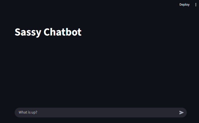
### Streamlit Interface ###
st.title("Sassy Chatbot")
Test your app by running this in your terminal:
streamlit run app.pyYour default browser should open showing your web app with the title "Sassy Chatbot." Notice the auto-reload feature; when you save changes, Streamlit prompts you to rerun the app.
Learning Insight: Streamlit uses "magic" rendering. You don't need to explicitly display elements. Simply calling st.title() automatically renders the title in your web interface.
Part 2: Building the Control Panel
Real applications need user controls. Let's add a sidebar with personality options and parameter controls.
Add this after your title:
# Sidebar controls
st.sidebar.header("Options")
st.sidebar.write("This is a demo of a sassy chatbot using OpenAI's API.")
# Temperature and token controls
max_tokens = st.sidebar.slider("Max Tokens", 1, 250, 100)
temperature = st.sidebar.slider("Temperature", 0.0, 1.0, 0.7)
# Personality selection
system_message_type = st.sidebar.selectbox("System Message",
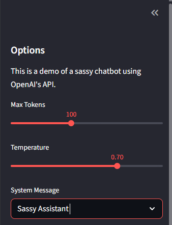
("Sassy Assistant", "Angry Assistant", "Custom"))Save and watch your sidebar populate with interactive controls. These sliders automatically store their values in the respective variables when users interact with them.
Adding Dynamic Personality System
Now let's make the personality selection actually work:
# Dynamic system prompt based on selection
if system_message_type == "Sassy Assistant":
    SYSTEM_PROMPT = "You are a sassy assistant that is fed up with answering questions."
elif system_message_type == "Angry Assistant":
    SYSTEM_PROMPT = "You are an angry assistant that likes yelling in all caps."
elif system_message_type == "Custom":
    SYSTEM_PROMPT = st.sidebar.text_area("Custom System Message",
        "Enter your custom system message here.")
else:
    SYSTEM_PROMPT = "You are a helpful assistant."
The custom option creates a text area where users can write their own personality instructions. Try switching between personalities and notice how the interface adapts.
Part 3: Understanding Session State
Here's where Streamlit gets tricky. Every time a user interacts with your app, Streamlit reruns the entire script from top to bottom. This would normally reset your chat history every time, which is not what we want for a conversation!
Session state solves this by persisting data across app reruns:
# Initialize session state for conversation memory
if "messages" not in st.session_state:
    st.session_state.messages = [{"role": "system", "content": SYSTEM_PROMPT}]
This creates a persistent messages list that survives app reruns. Now we need to modify our chat function to use session state:
def chat(user_input, temperature=TEMPERATURE, max_tokens=MAX_TOKENS):
    # Get messages from session state
    messages = st.session_state.messages
    messages.append({"role": "user", "content": user_input})

    enforce_token_budget(messages)

    # Add loading spinner for better UX
    with st.spinner("Thinking..."):
        response = client.chat.completions.create(
            model=MODEL,
            messages=messages,
            temperature=temperature,
            max_tokens=max_tokens
        )

    reply = response.choices[0].message.content
    messages.append({"role": "assistant", "content": reply})
    return reply
Learning Insight: Session state is like a dictionary that persists between app reruns. Think of it as your app's memory system.
Part 4: Interactive Buttons and Controls
Let's add buttons to make the interface more user-friendly:
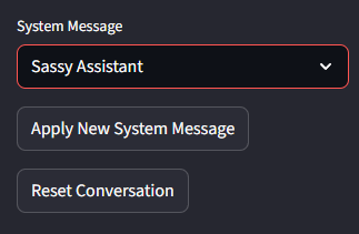
# Control buttons
if st.sidebar.button("Apply New System Message"):
    st.session_state.messages[0] = {"role": "system", "content": SYSTEM_PROMPT}
    st.success("System message updated.")

if st.sidebar.button("Reset Conversation"):
    st.session_state.messages = [{"role": "system", "content": SYSTEM_PROMPT}]
    st.success("Conversation reset.")
These buttons provide immediate feedback with success messages, creating a more polished user experience.
Part 5: The Chat Interface
Now for the main event—the actual chat interface. Add this code:
# Chat input using walrus operator
if prompt := st.chat_input("What is up?"):
    reply = chat(prompt, temperature=temperature, max_tokens=max_tokens)

# Display chat history
for message in st.session_state.messages[1:]:  # Skip system message
    with st.chat_message(message["role"]):
        st.markdown(message["content"])
The chat_input widget creates a text box at the bottom of your app. The walrus operator (:=) assigns the user input to prompt and checks if it exists in one line.
Visual Enhancement: Streamlit automatically adds user and assistant icons to chat messages when you use the proper role names ("user" and "assistant").
Part 6: Testing Your Complete App
Save your file and test the complete interface:
- Personality Test: Switch between Sassy and Angry assistants, apply the new system message, then chat to see the difference
- Memory Test: Have a conversation, then reference something you said earlier
- Parameter Test: Drag the max tokens slider to 1 and see how responses get cut off
- Reset Test: Use the reset button to clear conversation history
Your complete working app should look something like this:
import os
from openai import OpenAI
import tiktoken
import streamlit as st

# API and model configuration
api_key = st.secrets.get("OPENAI_API_KEY") or os.getenv("OPENAI_API_KEY")
client = OpenAI(api_key=api_key)
MODEL = "gpt-4o-mini"
TEMPERATURE = 0.7
MAX_TOKENS = 100
TOKEN_BUDGET = 1000
SYSTEM_PROMPT = "You are a fed up and sassy assistant who hates answering questions."

# [Token management functions here - same as starter code]

def chat(user_input, temperature=TEMPERATURE, max_tokens=MAX_TOKENS):
    messages = st.session_state.messages
    messages.append({"role": "user", "content": user_input})
    enforce_token_budget(messages)

    with st.spinner("Thinking..."):
        response = client.chat.completions.create(
            model=MODEL,
            messages=messages,
            temperature=temperature,
            max_tokens=max_tokens
        )

    reply = response.choices[0].message.content
    messages.append({"role": "assistant", "content": reply})
    return reply

### Streamlit Interface ###
st.title("Sassy Chatbot")
st.sidebar.header("Options")
st.sidebar.write("This is a demo of a sassy chatbot using OpenAI's API.")

max_tokens = st.sidebar.slider("Max Tokens", 1, 250, 100)
temperature = st.sidebar.slider("Temperature", 0.0, 1.0, 0.7)
system_message_type = st.sidebar.selectbox("System Message",
    ("Sassy Assistant", "Angry Assistant", "Custom"))

if system_message_type == "Sassy Assistant":
    SYSTEM_PROMPT = "You are a sassy assistant that is fed up with answering questions."
elif system_message_type == "Angry Assistant":
    SYSTEM_PROMPT = "You are an angry assistant that likes yelling in all caps."
elif system_message_type == "Custom":
    SYSTEM_PROMPT = st.sidebar.text_area("Custom System Message",
        "Enter your custom system message here.")

if "messages" not in st.session_state:
    st.session_state.messages = [{"role": "system", "content": SYSTEM_PROMPT}]

if st.sidebar.button("Apply New System Message"):
    st.session_state.messages[0] = {"role": "system", "content": SYSTEM_PROMPT}
    st.success("System message updated.")

if st.sidebar.button("Reset Conversation"):
    st.session_state.messages = [{"role": "system", "content": SYSTEM_PROMPT}]
    st.success("Conversation reset.")

if prompt := st.chat_input("What is up?"):
    reply = chat(prompt, temperature=temperature, max_tokens=max_tokens)

for message in st.session_state.messages[1:]:
    with st.chat_message(message["role"]):
        st.markdown(message["content"])
Part 7: Deploying to the Internet
Running locally is great for development, but deployment makes your project shareable and accessible to others. Streamlit Community Cloud offers free hosting directly from your GitHub repository.
Prepare for Deployment
First, create the required files in your project folder:
requirements.txt:
openai
streamlit
tiktoken.gitignore:
.streamlit/Note that if you’ve stored your API key in a .env file you should add this to .gitignore as well.
Secrets Management: Create a .streamlit/secrets.toml file locally:
OPENAI_API_KEY = "your-api-key-here"Important: Add .streamlit/ to your .gitignore so you don't accidentally commit your API key to GitHub.
GitHub Setup
- Create a new GitHub repository
- Push your code (the
.gitignorewill protect your secrets) - Your repository should contain:
app.py,requirements.txt, and.gitignore
Deploy to Streamlit Cloud
-
Go to share.streamlit.io
-
Connect your GitHub account
-
Select your repository and main branch
-
Choose your app file (
app.py) -
In Advanced settings, add your API key as a secret:
OPENAI_API_KEY = "your-api-key-here" -
Click "Deploy"
Within minutes, your app will be live at a public URL that you can share with anyone!
Security Note: The secrets you add in Streamlit Cloud are encrypted and secure. Never put API keys directly in your code files.
Understanding Key Concepts
Session State Deep Dive
Session state is Streamlit's memory system. Without it, every user interaction would reset your app completely. Think of it as a persistent dictionary that survives app reruns:
# Initialize once
if "my_data" not in st.session_state:
    st.session_state.my_data = []

# Use throughout your app
st.session_state.my_data.append("new item")
The Streamlit Execution Model
Streamlit reruns your entire script on every interaction. This "reactive" model means:
- Your app always shows the current state
- You need session state for persistence
- Expensive operations should be cached or minimized
Widget State Management
Widgets (sliders, inputs, buttons) automatically manage their state:
- Slider values are always current
- Button presses trigger reruns
- Form inputs update in real-time
Troubleshooting Common Issues
- "No module named 'streamlit'": Install Streamlit with
pip install streamlit - API key errors: Verify your environment variables or Streamlit secrets are set correctly
- App won't reload: Check for Python syntax errors in your terminal output
- Session state not working: Ensure you're checking
if "key" not in st.session_state:before initializing - Deployment fails: Verify your
requirements.txtincludes all necessary packages
Extending Your Chatbot App
Immediate Enhancements
- File Upload: Let users upload documents for the chatbot to reference
- Export Conversations: Add a download button for chat history
- Usage Analytics: Track token usage and costs
- Multiple Chat Sessions: Support multiple conversation threads
Advanced Features
- User Authentication: Require login for personalized experiences
- Database Integration: Store conversations permanently
- Voice Interface: Add speech-to-text and text-to-speech
- Multi-Model Support: Let users choose different AI models
Business Applications
- Customer Service Bot: Deploy for client support with company-specific knowledge
- Interview Prep Tool: Create domain-specific interview practice bots
- Educational Assistant: Build tutoring bots for specific subjects
- Content Generator: Develop specialized writing assistants
Key Takeaways
Building web interfaces for AI applications demonstrates that you can bridge the gap between technical capability and user accessibility. Through this tutorial, you've learned:
Technical Skills:
- Streamlit fundamentals and reactive programming model
- Session state management for persistent applications
- Web deployment from development to production
- Integration patterns for AI APIs in web contexts
Professional Skills:
- Creating user-friendly interfaces for technical functionality
- Managing secrets and security in deployed applications
- Building portfolio-worthy projects that demonstrate real-world skills
- Understanding the path from prototype to production application
Strategic Understanding:
- Why web interfaces matter for AI applications
- How to make technical projects accessible to non-technical users
- The importance of user experience in AI application adoption
You now have a deployed chatbot application that showcases multiple in-demand skills: AI integration, web development, user interface design, and cloud deployment. This foundation prepares you to build more sophisticated applications and demonstrates your ability to create complete, user-facing AI solutions.
More Projects to Try
We have some other project walkthrough tutorials you may also enjoy:
- Project Tutorial: Build Your First Data Project
- Project Tutorial: Profitable App Profiles for the App Store and Google Play Markets
- Project Tutorial: Investigating Fandango Movie Ratings
- Project Tutorial: Analyzing New York City High School Data
- Project Tutorial: Analyzing Helicopter Prison Escapes Using Python
- Project Tutorial: Build A Python Word Guessing Game
- Project Tutorial: Predicting Heart Disease with Machine Learning
- Project Tutorial: Customer Segmentation Using K-Means Clustering
- Project Tutorial: Answering Business Questions Using SQL
- Project Tutorial: Predicting Insurance Costs with Linear Regression
- Project Tutorial: Analyzing Startup Fundraising Deals from Crunchbase
- Project Tutorial: Finding Heavy Traffic Indicators on I-94
- Project Tutorial: Star Wars Survey Analysis Using Python and Pandas
- Project Tutorial: Build an AI Chatbot with Python and the OpenAI API