PySpark pipelines that work beautifully with test data often crawl (or crash) in production. For example, a pipeline runs great at a small scale, with maybe a few hundred records finishing in under a minute. Then the company grows, and that same pipeline now processes hundreds of thousands of records and takes 45 minutes. Sometimes it doesn't finish at all. Your team lead asks, "Can you make this faster?"

In this tutorial, we’ll see how to systematically diagnose and fix those performance problems. We'll start with a deliberately unoptimized pipeline (47 seconds for just 75 records — yikes!), identify exactly what's slow using Spark's built-in tools, then fix it step-by-step until it runs in under 5 seconds. Same data, same hardware, just better code.

Before we start our optimization, let's set the stage. We've updated the ETL pipeline from the previous tutorial to use production-standard patterns, which means we're running everything in Docker with Spark's native parquet writers, just like you would in a real cluster environment. If you aren’t familiar with the previous tutorial, don’t worry! You can seamlessly jump into this one to learn pipeline optimization.

Getting the Starter Files

Let's get the starter files from our repository.

# Clone the full tutorials repo and navigate to this project
git clone <https://github.com/dataquestio/tutorials.git>
cd tutorials/pyspark-optimization-tutorial

This tutorial uses a local docker-compose.yml that exposes port 4040 for the Spark UI, so make sure you cloned the full repo, not just the subdirectory.

The starter files include:

• Baseline ETL pipeline code (in src/etl_pipeline.py and main.py)
• Sample grocery order data (in data/raw/)
• Docker configuration for running Spark locally
• Solution files for reference (in solution/)

Quick note: Spark 4.x enables Adaptive Query Execution (AQE) by default, which automatically handles some optimizations like dynamic partition coalescing. We've disabled it for this tutorial so you can see the raw performance problems clearly. Understanding these issues helps you write better code even when AQE is handling them automatically, which you'll re-enable in production.

Now, let's run this production-ready baseline to see what we’re dealing with.

Running the baseline

Make sure you're in the correct directory and start your Docker container with port access:

cd /tutorials/pyspark-optimization-tutorial
docker compose run --rm --service-ports lab

This opens an interactive shell inside the container. The --service-ports flag exposes port 4040, which you'll need to access Spark's web interface. We'll use that in a moment to see exactly what your pipeline is doing.

Inside the container, run:

python main.py

Pipeline completed in 47.15 seconds
WARNING: Total allocation exceeds 95.00% of heap memory
[...25 more memory warnings...]

47 seconds for 75 records. Look at those memory warnings! Spark is struggling because we're creating way too many partition files. We're scanning the data multiple times for simple counts. We're doing expensive aggregations without any caching. Every operation triggers a full pass through the data.

The good news? These are common, fixable mistakes. We'll systematically identify and eliminate them until this runs in under 5 seconds. Let's start by diagnosing exactly what's slow.

Understanding What's Slow: The Spark UI

We can't fix performance problems by guessing. The first rule of optimization: measure, then fix.

Spark gives us a built-in diagnostic tool that shows exactly what our pipeline is doing. It's called the Spark UI, and it runs every time you execute a Spark job. For this tutorial, we've added a pause at the end of our main.py job so you can explore the Spark UI. In production, you'd use Spark's history server to review completed jobs, but for learning, this pause lets you click around and build familiarity with the interface.

Accessing the Spark UI

Remember that port 4040 we exposed with our Docker command? Now we're going to use it. While your pipeline is running (or paused at the end), open a browser and go to http://localhost:4040.

You'll see Spark's web interface showing every job, stage, and task your pipeline executed. This is where you diagnose bottlenecks.

What to Look For

The Spark UI has a lot of tabs and metrics, which can feel overwhelming. For our work today we’ll focus on three things:

The Jobs tab shows every action that triggered execution. Each .count() or .write() creates a job. If you see 20+ jobs for a simple pipeline, you're doing too much work.

Stage durations tell you where time is being spent. Click into a job to see its stages. Spending 30 seconds on a count operation for 75 records? That's a bottleneck.

Number of tasks reveals partitioning problems. See 200 tasks to process 75 records? That's way too much overhead.

Reading the Baseline Pipeline

Open the Jobs tab. You'll see a table that looks messier than you'd expect:

Job Id  Description                                     Duration
0       count at NativeMethodAccessorImpl.java:0        0.5 s
1       count at NativeMethodAccessorImpl.java:0        0.1 s
2       count at NativeMethodAccessorImpl.java:0        0.1 s
...
13      parquet at NativeMethodAccessorImpl.java:0      3 s
15      parquet at NativeMethodAccessorImpl.java:0      2 s
19      collect at etl_pipeline.py:195                  0.3 s
20      collect at etl_pipeline.py:201                  0.3 s

The descriptions aren't particularly helpful, but count them. 22 jobs total. That's a lot of work for 75 records!

Most of these are count operations. Every time we logged a count in our code, Spark had to scan the entire dataset. Jobs 0-12 are all those .count() calls scattered through extraction and transformation. That's inefficiency #1.

Jobs 13 and 15 are our parquet writes. If you click into job 13, you'll see it created around 200 tasks to write 75 records. That's why we got all those memory warnings: too many tiny files means too much overhead.

Jobs 19 and 20 are the collect operations from our summary report (you can see the line numbers: etl_pipeline.py:195 and :201). Each one triggers more computation.

The Spark UI isn't always pretty, but it's showing us exactly what's wrong:

• 22 jobs for a simple pipeline - way too much work
• Most jobs are counts - rescanning data repeatedly
• 200 tasks to write 75 records - partitioning gone wrong
• Separate collection operations - no reuse of computed data

You don't need to understand every Java stack trace; you just need to count the jobs, spot the repeated operations, and identify where time is being spent. That's enough to know what to fix.

Eliminating Redundant Operations

Look back at those 22 jobs in the Spark UI. Most of them are counts. Every time we wrote df.count() to log how many records we had, Spark scanned the entire dataset. Right now, that's just 75 records, but scale to 75 million, and those scans eat hours of runtime.

Spark is lazy by design, so transformations like .filter() and .withColumn() build a plan but don't actually do anything. Only actions like .count(), .collect(), and .write() trigger execution. Usually, this is good because Spark can optimize the whole plan at once, but when you sprinkle counts everywhere "just to see what's happening," you're forcing Spark to execute repeatedly.

The Problem: Logging Everything

Open src/etl_pipeline.py and look at the extract_sales_data function:

def extract_sales_data(spark, input_path):
    """Read CSV files with explicit schema"""

    logger.info(f"Reading sales data from {input_path}")

    # ... schema definition ...

    df = spark.read.csv(input_path, header=True, schema=schema)

    # PROBLEM: This forces a full scan just to log the count
    logger.info(f"Loaded {df.count()} records from {input_path}")

    return df

That count seems harmless because we want to know how many records we loaded, right? But we're calling this function three times (once per CSV file), so that's three full scans before we've done any actual work.

Now look at extract_all_data:

def extract_all_data(spark):
    """Combine data from multiple sources"""

    online_orders = extract_sales_data(spark, "data/raw/online_orders.csv")
    store_orders = extract_sales_data(spark, "data/raw/store_orders.csv")
    mobile_orders = extract_sales_data(spark, "data/raw/mobile_orders.csv")

    all_orders = online_orders.unionByName(store_orders).unionByName(mobile_orders)

    # PROBLEM: Another full scan right after combining
    logger.info(f"Combined dataset has {all_orders.count()} orders")

    return all_orders

We just scanned three times to count individual files, then scanned again to count the combined result. That's four scans before we've even started transforming data.

The Fix: Count Only What Matters

Only count when you need the number for business logic, not for logging convenience.

Remove the counts from extract_sales_data:

def extract_sales_data(spark, input_path):
    """Read CSV files with explicit schema"""

    logger.info(f"Reading sales data from {input_path}")

    schema = StructType([
        StructField("order_id", StringType(), True),
        StructField("customer_id", StringType(), True),
        StructField("product_name", StringType(), True),
        StructField("price", StringType(), True),
        StructField("quantity", StringType(), True),
        StructField("order_date", StringType(), True),
        StructField("region", StringType(), True)
    ])

    df = spark.read.csv(input_path, header=True, schema=schema)

    # No count here - just return the DataFrame
    return df

Remove the count from extract_all_data:

def extract_all_data(spark):
    """Combine data from multiple sources"""

    online_orders = extract_sales_data(spark, "data/raw/online_orders.csv")
    store_orders = extract_sales_data(spark, "data/raw/store_orders.csv")
    mobile_orders = extract_sales_data(spark, "data/raw/mobile_orders.csv")

    all_orders = online_orders.unionByName(store_orders).unionByName(mobile_orders)

    logger.info("Combined data from all sources")
    return all_orders

Fixing the Transform Phase

Now look at remove_test_data and handle_duplicates. Both calculate how many records they removed:

def remove_test_data(df):
    """Filter out test records"""
    df_filtered = df.filter(
        ~(upper(col("customer_id")).contains("TEST") |
          upper(col("product_name")).contains("TEST") |
          col("customer_id").isNull() |
          col("order_id").isNull())
    )

    # PROBLEM: Two counts just to log the difference
    removed_count = df.count() - df_filtered.count()
    logger.info(f"Removed {removed_count} test/invalid orders")

    return df_filtered

That's two full scans (one for df.count(), one for df_filtered.count()) just to log a number. Here's the fix:

def remove_test_data(df):
    """Filter out test records"""
    df_filtered = df.filter(
        ~(upper(col("customer_id")).contains("TEST") |
          upper(col("product_name")).contains("TEST") |
          col("customer_id").isNull() |
          col("order_id").isNull())
    )

    logger.info("Removed test and invalid orders")
    return df_filtered

Do the same for handle_duplicates:

def handle_duplicates(df):
    """Remove duplicate orders"""
    df_deduped = df.dropDuplicates(["order_id"])

    logger.info("Removed duplicate orders")
    return df_deduped

Counts make sense during development when we're validating logic. Feel free to add them liberally - check that your test filter actually removed 10 records, verify deduplication worked. But once the pipeline works? Remove them before deploying to production, where you'd use Spark's accumulators or monitoring systems instead.

Keeping One Strategic Count

Let's keep exactly one count operation in main.py after the full transformation completes. This tells us the final record count without triggering excessive scans during processing:

def main():
    # ... existing code ...

    try:
        spark = create_spark_session()
        logger.info("Spark session created")

        # Extract
        raw_df = extract_all_data(spark)
        logger.info("Extracted raw data from all sources")

        # Transform
        clean_df = transform_orders(raw_df)
        logger.info(f"Transformation complete: {clean_df.count()} clean records")

        # ... rest of pipeline ...

One count at a key checkpoint. That's it.

What About the Summary Report?

Look at what create_summary_report is doing:

total_orders = df.count()
unique_customers = df.select("customer_id").distinct().count()
unique_products = df.select("product_name").distinct().count()
total_revenue = df.agg(sum("total_amount")).collect()[0][0]
# ... more separate operations ...

Each line scans the data independently - six separate scans for six metrics. We'll fix this properly in a later section when we talk about efficient aggregations, but for now, let's just remove the call to create_summary_report from main.py entirely. Comment it out:

        load_to_parquet(clean_df, output_path)
        load_to_parquet(metrics_df, metrics_path)

        # summary = create_summary_report(clean_df)  # Temporarily disabled

        runtime = (datetime.now() - start_time).total_seconds()
        logger.info(f"Pipeline completed in {runtime:.2f} seconds")

Test the Changes

Run your optimized pipeline:

python main.py

Watch the output. You'll see far fewer log messages because we're not counting everything. More importantly, check the completion time:

Pipeline completed in 42.70 seconds

We just shaved off 5 seconds by removing unnecessary counts.

Not a massive win, but we're just getting started. More importantly, check the Spark UI (http://localhost:4040) and you should see fewer jobs now, maybe 12-15 instead of 22.

Not all optimizations give massive speedups, but fixing them systematically adds up. We removed unnecessary work, which is always good practice. Now let's tackle the real problem: partitioning.

Fixing Partitioning: Right-Sizing Your Data

When Spark processes data, it splits it into chunks called partitions. Each partition gets processed independently, potentially on different machines or CPU cores. This is how Spark achieves parallelism. But Spark doesn't automatically know the perfect number of partitions for your data.

By default, Spark often creates 200 partitions for operations like shuffles and writes. That's a reasonable default if you're processing hundreds of gigabytes across a 50-node cluster, but we're processing 75 records on a single machine. Creating 200 partition files means:

• 200 tiny files written to disk
• 200 file handles opened simultaneously
• Memory overhead for managing 200 separate write operations
• More time spent on coordination than actual work

It's like hiring 200 people to move 75 boxes. Most of them stand around waiting while a few do all the work, and you waste money coordinating everyone.

Seeing the Problem

Open the Spark UI and look at the Stages tab. Find one of the parquet write stages (you'll see them labeled parquet at NativeMethodAccessorImpl.java:0).

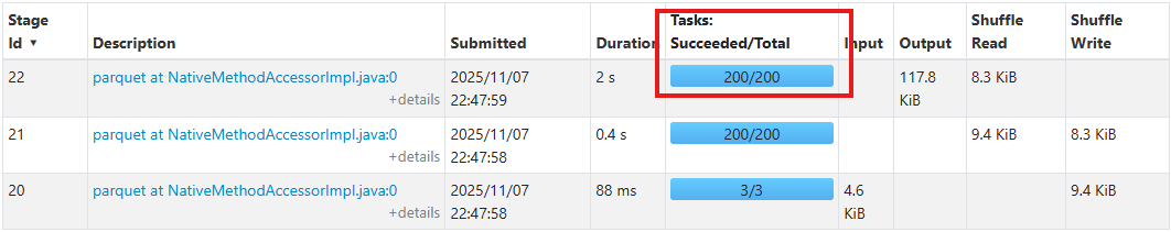
Look at the Tasks: Succeeded/Total column and you'll see 200/200. Spark created 200 separate tasks to write 75 records. Now, look at the Shuffle Write column, which is probably showing single-digit kilobytes. We're using massive parallelism for tiny amounts of data.

Each of those 200 tasks creates overhead: opening a file handle, coordinating with the driver, writing a few bytes, then closing. Most tasks spend more time on coordination than actual work.

The Fix: Coalesce

We need to reduce the number of partitions before writing. Spark gives us two options: repartition() and coalesce().

Repartition does a full shuffle - redistributes all data across the cluster. It's expensive but gives you exact control.

Coalesce is smarter. It combines existing partitions without shuffling. If you have 200 partitions and coalesce to 2, Spark just merges them in place, which is much faster.

For our data size, we want 1 partition - one file per output, clean and simple.

Update load_to_parquet in src/etl_pipeline.py:

def load_to_parquet(df, output_path):
    """Save to parquet with proper partitioning"""

    logger.info(f"Writing data to {output_path}")

    # Coalesce to 1 partition before writing
    # This creates a single output file instead of 200 tiny ones
    df.coalesce(1) \
      .write \
      .mode("overwrite") \
      .parquet(output_path)

    logger.info(f"Successfully wrote data to {output_path}")

When to Use Different Partition Counts

You don’t always want one partition. Here's when to use different counts:

For small datasets (under 1GB): Use 1-4 partitions. Minimize overhead.

For medium datasets (1-10GB): Use 10-50 partitions. Balance parallelism and overhead.

For large datasets (100GB+): Use 100-500 partitions. Maximize parallelism.

General guideline: Aim for 128MB to 1GB per partition. That's the sweet spot where each task has enough work to justify the overhead but not so much that it runs out of memory.

For our 75 records, 1 partition works perfectly. In production environments, AQE typically handles this partition sizing automatically, but understanding these principles helps you write better code even when AQE is doing the heavy lifting.

Test the Fix

Run the pipeline again:

python main.py

Those memory warnings should be gone. Check the timing:

Pipeline completed in 20.87 seconds

We just saved another 22 seconds by fixing partitioning. That's cutting our runtime in half. From 47 seconds in the original baseline to 20 seconds now, and we've only made two changes.

Check the Spark UI Stages tab. Now your parquet write stages should show 1/1 or 2/2 tasks instead of 200/200.

Look at your output directory:

ls data/processed/orders/

Before, you'd see hundreds of tiny parquet files with names like part-00001.parquet, part-00002.parquet, and so on. Now you'll see one clean file.

Why This Matters at Scale

Wrong partitioning breaks pipelines at scale. With 75 million records, having too many partitions creates coordination overhead. Having too few means you can't parallelize. And if your data is unevenly distributed (some partitions with 1 million records, others with 10,000), you get stragglers, slow tasks that hold up the entire job while everyone else waits.

Get partitioning right and your pipeline uses less memory, produces cleaner files, performs better downstream, and scales without crashing.

We've cut our runtime in half by eliminating redundant work and fixing partitioning. Next up: caching. We're still recomputing DataFrames multiple times, and that's costing us time. Let's fix that.

Strategic Caching: Stop Recomputing the Same Data

Here's a question: how many times do we use clean_df in our pipeline?

Look at main.py:

clean_df = transform_orders(raw_df)
logger.info(f"Transformation complete: {clean_df.count()} clean records")

metrics_df = create_metrics(clean_df)  # Using clean_df here
logger.info(f"Generated {metrics_df.count()} metric records")

load_to_parquet(clean_df, output_path)  # Using clean_df again
load_to_parquet(metrics_df, metrics_path)

We use clean_df three times: once for the count, once to create metrics, and once to write it. Here's the catch: Spark recomputes that entire transformation pipeline every single time.

Remember, transformations are lazy. When you write clean_df = transform_orders(raw_df), Spark doesn't actually clean the data. It just creates a plan: "When someone needs this data, here's how to build it." Every time you use clean_df, Spark goes back to the raw CSVs, reads them, applies all your transformations, and produces the result. Three uses = three complete executions.

That's wasteful.

The Solution: Cache It

Caching tells Spark: "I'm going to use this DataFrame multiple times. Compute it once, keep it in memory, and reuse it."

Update main.py to cache clean_df after transformation:

def main():
    # ... existing code ...

    try:
        spark = create_spark_session()
        logger.info("Spark session created")

        # Extract
        raw_df = extract_all_data(spark)
        logger.info("Extracted raw data from all sources")

        # Transform
        clean_df = transform_orders(raw_df)

        # Cache because we'll use this multiple times
        clean_df.cache()

        logger.info(f"Transformation complete: {clean_df.count()} clean records")

        # Create aggregated metrics
        metrics_df = create_metrics(clean_df)
        logger.info(f"Generated {metrics_df.count()} metric records")

        # Load
        output_path = "data/processed/orders"
        metrics_path = "data/processed/metrics"

        load_to_parquet(clean_df, output_path)
        load_to_parquet(metrics_df, metrics_path)

        # Clean up the cache when done
        clean_df.unpersist()

        runtime = (datetime.now() - start_time).total_seconds()
        logger.info(f"Pipeline completed in {runtime:.2f} seconds")

We added clean_df.cache() right after transformation and clean_df.unpersist() when we're done with it.

What Actually Happens

When you call .cache(), nothing happens immediately. Spark just marks that DataFrame as "cacheable." The first time you actually use it (the count operation), Spark computes the result and stores it in memory. Every subsequent use pulls from memory instead of recomputing.

The .unpersist() at the end frees up that memory. Not strictly necessary (Spark will eventually evict cached data when it needs space), but it's good practice to be explicit.

When to Cache (and When Not To)

Not every DataFrame needs caching. Use these guidelines:

Cache when:

• You use a DataFrame 2+ times
• The DataFrame is expensive to compute
• It's reasonably sized (Spark will spill to disk if it doesn't fit in memory, but excessive spilling hurts performance)

Don't cache when:

• You only use it once (wastes memory for no benefit)
• Computing it is cheaper than the cache overhead (very simple operations)
• You're caching so much data that Spark is constantly evicting and re-caching (check the Storage tab in Spark UI to see if this is happening)

For our pipeline, caching clean_df makes sense because we use it three times and it's small. Caching the raw data wouldn't help because we only transform it once.

Test the Changes

Run the pipeline:

python main.py

Check the timing:

Pipeline completed in 18.11 seconds

We saved about 3 seconds with caching. Want to see what actually got cached? Check the Storage tab in the Spark UI to see how much data is in memory versus what has been spilled to disk. For our small dataset, everything should be in memory.

From 47 seconds at baseline to 18 seconds now — that's a 62% improvement from three optimizations: removing redundant counts, fixing partitioning, and caching strategically.

The performance gain from caching is smaller than partitioning because our dataset is tiny. With larger data, caching makes a much bigger difference.

Too Much Caching

Caching isn't free. It uses memory, and if you cache too much, Spark starts evicting data to make room for new caches. This causes thrashing, constant cache evictions and recomputations, which makes everything slower.

Cache strategically. If you'll use it more than once, cache it. If not, don't.

We've now eliminated redundant operations, fixed partitioning, and added strategic caching. Next up: filtering early. We're still cleaning all the data before removing test records, which is backwards. Let's fix that.

Filter Early: Don't Clean Data You'll Throw Away

Look at our transformation pipeline in transform_orders:

def transform_orders(df):
    """Apply all transformations in sequence"""

    logger.info("Starting data transformation...")

    df = clean_customer_id(df)
    df = clean_price_column(df)
    df = standardize_dates(df)
    df = remove_test_data(df)       # ← This should be first!
    df = handle_duplicates(df)

See the problem? We're cleaning customer IDs, parsing prices, and standardizing dates for all the records. Then, at the end, we remove test data and duplicates. We just wasted time cleaning data we're about to throw away.

It's like washing dirty dishes before checking which ones are broken. Why scrub something you're going to toss?

Why This Matters

Test data removal and deduplication are cheap operations because they're just filters. Price cleaning and date parsing are expensive because they involve regex operations and type conversions on every row.

Right now we're doing expensive work on 85 records, then filtering down to 75. We should filter to 75 first, then do expensive work on just those records.

With our tiny dataset, this won't save much time. But imagine production: you load 10 million records, 5% are test data and duplicates. That's 500,000 records you're cleaning for no reason. Early filtering means you only clean 9.5 million records instead of 10 million. That's real time saved.

The Fix: Reorder Transformations

Move the filters to the front. Change transform_orders to:

def transform_orders(df):
    """Apply all transformations in sequence"""

    logger.info("Starting data transformation...")

    # Filter first - remove data we won't use
    df = remove_test_data(df)
    df = handle_duplicates(df)

    # Then do expensive transformations on clean data only
    df = clean_customer_id(df)
    df = clean_price_column(df)
    df = standardize_dates(df)

    # Cast quantity and add calculated fields
    df = df.withColumn(
        "quantity",
        when(col("quantity").isNotNull(), col("quantity").cast(IntegerType()))
        .otherwise(1)
    )

    df = df.withColumn("total_amount", col("unit_price") * col("quantity")) \
           .withColumn("processing_date", current_date()) \
           .withColumn("year", year(col("order_date"))) \
           .withColumn("month", month(col("order_date")))

    logger.info("Transformation complete")

    return df

The Principle: Push Down Filters

This is called predicate pushdown in database terminology, but the concept is simple: do your filtering as early as possible in the pipeline. Reduce your data size before doing expensive operations.

This applies beyond just test data:

• If you're only analyzing orders from 2024, filter by date right after reading
• If you only care about specific regions, filter by region immediately
• If you're joining two datasets and one is huge, filter both before joining

The general pattern: filter early, transform less.

Test the Changes

Run the pipeline:

python main.py

Check the timing:

Pipeline completed in 17.71 seconds

We saved about a second. In production with millions of records, early filtering can be the difference between a 10-minute job and a 2-minute job.

When Order Matters

Not all transformations can be reordered. Some have dependencies:

• You can't calculate total_amount before you've cleaned unit_price
• You can't extract the year from order_date before standardizing the date format
• You can't deduplicate before you've standardized customer IDs (or you might miss duplicates)

But filters that don't depend on transformations? Move those to the front.

Let's tackle one final improvement: making the summary report efficient.

Efficient Aggregations: Compute Everything in One Pass

Remember that summary report we commented out earlier? Let's bring it back and fix it properly.

Here's what create_summary_report currently does:

def create_summary_report(df):
    """Generate summary statistics"""

    logger.info("Generating summary report...")

    total_orders = df.count()
    unique_customers = df.select("customer_id").distinct().count()
    unique_products = df.select("product_name").distinct().count()
    total_revenue = df.agg(sum("total_amount")).collect()[0][0]

    date_stats = df.agg(
        min("order_date").alias("earliest"),
        max("order_date").alias("latest")
    ).collect()[0]

    region_count = df.groupBy("region").count().count()

    # ... log everything ...

Count how many times we scan the data. Six separate operations: count the orders, count distinct customers, count distinct products, sum revenue, get date range, and count regions. Each one reads through the entire DataFrame independently.

The Fix: Single Aggregation Pass

Spark lets you compute multiple aggregations in one pass. Here's how:

Replace create_summary_report with this optimized version:

def create_summary_report(df):
    """Generate summary statistics efficiently"""

    logger.info("Generating summary report...")

    # Compute everything in a single aggregation
    stats = df.agg(
        count("*").alias("total_orders"),
        countDistinct("customer_id").alias("unique_customers"),
        countDistinct("product_name").alias("unique_products"),
        sum("total_amount").alias("total_revenue"),
        min("order_date").alias("earliest_date"),
        max("order_date").alias("latest_date"),
        countDistinct("region").alias("regions")
    ).collect()[0]

    summary = {
        "total_orders": stats["total_orders"],
        "unique_customers": stats["unique_customers"],
        "unique_products": stats["unique_products"],
        "total_revenue": stats["total_revenue"],
        "date_range": f"{stats['earliest_date']} to {stats['latest_date']}",
        "regions": stats["regions"]
    }

    logger.info("\n=== ETL Summary Report ===")
    for key, value in summary.items():
        logger.info(f"{key}: {value}")
    logger.info("========================\n")

    return summary

One .agg() call, seven metrics computed. Spark scans the data once and calculates everything simultaneously.

Now uncomment the summary report call in main.py:

        load_to_parquet(clean_df, output_path)
        load_to_parquet(metrics_df, metrics_path)

        # Generate summary report
        summary = create_summary_report(clean_df)

        # Clean up the cache when done
        clean_df.unpersist()

How This Works

When you chain multiple aggregations in .agg(), Spark sees them all at once and creates a single execution plan. Everything gets calculated together in one pass through the data, not sequentially.

This is the difference between:

• Six passes: Read → count → Read → distinct customers → Read → distinct products...
• One pass: Read → count + distinct customers + distinct products + sum + min + max + regions

Same results, fraction of the work.

Test the Final Pipeline

Run it:

python main.py

Check the output:

=== ETL Summary Report ===
2025-11-07 23:14:22,285 - INFO - total_orders: 75
2025-11-07 23:14:22,285 - INFO - unique_customers: 53
2025-11-07 23:14:22,285 - INFO - unique_products: 74
2025-11-07 23:14:22,285 - INFO - total_revenue: 667.8700000000003
2025-11-07 23:14:22,285 - INFO - date_range: 2024-10-15 to 2024-11-10
2025-11-07 23:14:22,285 - INFO - regions: 4
2025-11-07 23:14:22,286 - INFO - ========================

2025-11-07 23:14:22,297 - INFO - Pipeline completed in 18.28 seconds

We're at 18 seconds. Adding the efficient summary back added less than a second because it computes everything in one pass. The old version with six separate scans would probably take 24+ seconds.

Before and After: The Complete Picture

Let's recap what we've done:

Baseline (47 seconds):

• Multiple counts scattered everywhere
• 200 partitions for 75 records
• No caching, constant recomputation
• Test data removed after expensive transformations
• Summary report with six separate scans

Optimized (18 seconds):

• Strategic counting only where needed
• 1 partition per output file
• Cached frequently-used DataFrames
• Filters first, transformations second
• Summary report in a single aggregation

Result: 61% faster with the same hardware, same data, just better code.

And here's the thing: these optimizations scale. With 75,000 records instead of 75, the improvements would be even more dramatic. With 75 million records, proper optimization is the difference between a job that completes and one that crashes.

You've now seen the core optimization techniques that solve most real-world performance problems. Let's wrap up with what you've learned and when to apply these patterns.

What You've Accomplished

You can diagnose performance problems. The Spark UI showed you exactly where time was being spent. Too many jobs meant redundant operations. Too many tasks meant partitioning problems. Now you know how to read those signals.

You know when and how to optimize. Remove unnecessary work first. Fix obvious problems, such as incorrect partition counts. Cache strategically when data gets reused. Filter early to reduce data volume. Combine aggregations into single passes. Each technique targets a specific bottleneck.

You understand the tradeoffs. Caching uses memory. Coalescing reduces parallelism. Different situations need different techniques. Pick the right ones for your problem.

You learned the process: measure, identify bottlenecks, fix them, measure again. That process works whether you're optimizing a 75-record tutorial or a production pipeline processing terabytes.

When to Apply These Techniques

Don't optimize prematurely. If your pipeline runs in 30 seconds and runs once a day, it's fine. Spend your time building features instead of shaving seconds.

Optimize when:

• Your pipeline can't finish before the next run starts
• You're hitting memory limits or crashes
• Jobs are taking hours when they should take minutes
• You're paying significant cloud costs for compute time

Then follow the process you just learned: measure what's slow, fix the biggest bottleneck, measure again. Repeat until it's fast enough.

What's Next

You've optimized a single-machine pipeline. The next tutorial covers integrating PySpark with the broader big data ecosystem: connecting to data warehouses, working with cloud storage, orchestrating with Airflow, and understanding when to scale to a real cluster.

Before you move on to distributed clusters and ecosystem integration, take what you've learned and apply it. Find a slow Spark job - at work, in a project, or just a dataset you're curious about. Profile it with the Spark UI. Apply these optimizations. See the improvement for yourself.

In production, enable AQE (spark.sql.adaptive.enabled = true) and let Spark's automatic optimizations work alongside your manual tuning.

One Last Thing

Performance optimization feels intimidating when you're starting out. It seems like it requires deep expertise in Spark internals, JVM tuning, and cluster configuration.

But as you just saw, most performance problems come from a handful of common mistakes. Unnecessary operations. Wrong partitioning. Missing caches. Poor filtering strategies. Fix those, and you've solved 80% of real-world performance issues.

You don't need to be a Spark expert to write fast code. You need to understand what Spark is doing, identify the waste, and eliminate it. That's exactly what you did today.

Now go make something fast.

This guide helps you set up a clean, isolated environment for running Dataquest tutorials. While many tutorials work fine directly on your computer, some (particularly those involving data processing tools like PySpark) can run into issues depending on your operating system or existing software setup. The lab environment we'll create ensures everything runs consistently, with the right versions of Python and other tools, without affecting your main system.

What's a Lab Environment?

You can think of this "lab" as a separate workspace just for your Dataquest tutorials. It's a controlled space where you can experiment and test code without affecting your main computer. Just like scientists use labs for experiments, we'll use this development lab to work through tutorials safely.

Benefits for everyone:

• Windows/Mac users: Avoid errors from system differences. No more "command not found" or PySpark failing to find files
• Linux users: Get the exact versions of Python and Java needed for tutorials, without conflicting with your system's packages
• Everyone: Keep your tutorial work separate from personal projects. Your code and files are saved normally, but any packages you install or system changes you make stay contained in the lab

We'll use a tool called Docker to create this isolated workspace. Think of it as having a dedicated computer just for tutorials inside your regular computer. Your files and code are saved just like normal (you can edit them with your favorite editor), but the tutorial environment itself stays clean and separate from everything else on your system.

The lab command you'll use creates this environment, and it mirrors real data engineering workflows (most companies use isolated environments like this to ensure consistency across their teams).

Installing Docker

Docker creates isolated Linux environments on any operating system. This means you'll get a consistent Linux workspace whether you're on Windows, Mac, or even Linux itself. We're using it as a simple tool, so no container orchestration or cloud deployment knowledge is needed.

On Windows:
Download Docker Desktop from docker.com/products/docker-desktop. Run the installer, restart your computer when prompted, and open Docker Desktop. You'll see a whale icon in your system tray when it's running.

Note: Docker Desktop will automatically enable required Windows features like WSL 2. If you see an error about virtualization, you may need to enable it in your computer's BIOS settings. Search online for your computer model + "enable virtualization" for specific steps.

On Mac:
Download Docker Desktop for your chip type (Intel or Apple Silicon) from the same link. Drag Docker to your Applications folder and launch it. You'll see the whale in your menu bar.

On Linux:
You probably already have Docker, but if not, run this command in your terminal:

curl -fsSL https://get.docker.com -o get-docker.sh && sh get-docker.sh

Verify it works:
Open your terminal (PowerShell, Terminal, or bash) and run:

docker --version
docker compose version

You should see version numbers for both commands. If you see "command not found," restart your terminal or computer and try again.

Getting the Lab Environment

The lab is already configured in the Dataquest tutorials repository. Clone or download it:

git clone https://github.com/dataquestio/tutorials.git
cd tutorials

If you don't have git, download the repository as a ZIP file from GitHub and extract it.

The repository includes everything you need:

• Dockerfile - Configures the Linux environment with Python 3.11 and Java (for Spark)
• docker-compose.yml - Defines the lab setup
• Tutorial folders with all the code and data

Starting Your Lab

In your IDE’s terminal, ensure you’re in the tutorials folder and start the lab:

docker compose run --rm lab

Note that the first time you run this command, the setup may take 2-5 minutes.

You're now in Linux! Your prompt will change to something like root@abc123:/tutorials#, which is your Linux command line where everything will work as expected.

The --rm flag means the lab cleans itself up when you exit, keeping your system tidy.

Using Your Lab

Once you’re in the lab environment, here's your typical workflow:

1. Navigate to the tutorial you're working on

# See all available tutorials
ls

# Enter a specific tutorial
cd pyspark-etl

2. Install packages as needed
Each tutorial might need different packages:

# For PySpark tutorials
pip install pyspark

# For data manipulation tutorials
pip install pandas numpy

# For database connections
pip install sqlalchemy psycopg2-binary

3. Run the tutorial code

python <script-name>.py

Because the code will run within a standardized Linux environment, you shouldn’t run into setup errors.

4. Edit files normally
The beauty of this setup: you can still use your favorite editor! The tutorials folder on your computer is synchronized with the lab. Edit files in VS Code, PyCharm, or any editor, and the lab sees changes immediately.

5. Exit when done
Type exit or press Ctrl+D to leave the lab. The environment cleans itself up automatically.

Common Workflow Examples

Running a PySpark tutorial:

docker compose run --rm lab
cd pyspark-etl
pip install pyspark pandas
python main.py

Working with Jupyter notebooks:

docker compose run --rm -p 8888:8888 lab
pip install jupyterlab
jupyter lab --ip=0.0.0.0 --allow-root --no-browser
# Open the URL it shows in your browser

Keeping packages installed between sessions:
If you're tired of reinstalling packages, create a requirements file:

# After installing packages, save them
pip freeze > requirements.txt

# Next session, restore them
pip install -r requirements.txt

Quick Reference

The one command you need:

# From the tutorials folder
docker compose run --rm lab

Exit the lab:

exit # Or press Ctrl+D

Where things are:

• Tutorial code: Each folder in /tutorials
• Your edits: Automatically synchronized
• Data files: In each tutorial's data/ folder
• Output files: Save to the tutorial folder to see them on your computer

Adding services (databases, etc.):
For tutorials needing PostgreSQL, MongoDB, or other services, we can extend the docker-compose.yml. For now, the base setup handles all Python and PySpark tutorials.

Troubleshooting

• "Cannot connect to Docker daemon"

  • Docker Desktop needs to be running. Start it from your applications.

• "docker compose" not recognized

  • Older Docker versions use docker-compose (with a hyphen). Try:

    docker-compose run --rm lab

• Slow performance on Windows

  • Docker on Windows can be slow with large datasets. For better performance, store data files in the container rather than the mounted folder.

• "Permission denied" on Linux

  • Add your user to the docker group:

    sudo usermod -aG docker $USER

    Then log out and back in.

You're Ready

You now have a Linux lab environment that matches production systems. Happy experimenting!

You've learned PySpark basics: RDDs, DataFrames, maybe some SQL queries. You can transform data and run aggregations in notebooks. But here's the thing: data engineering is about building pipelines that run reliably every single day, handling the messy reality of production data.

Today, we're building a complete ETL pipeline from scratch. This pipeline will handle the chaos you'll actually encounter at work: inconsistent date formats, prices with dollar signs, test data that somehow made it to production, and customer IDs that follow different naming conventions.

Here's the scenario: You just started as a junior data engineer at an online grocery delivery service. Your team lead drops by your desk with a problem. "Hey, we need help. Our daily sales report is a mess. The data comes in as CSVs from three different systems, nothing matches up, and the analyst team is doing everything manually in Excel. Can you build us an ETL pipeline?"

She shows you what she's dealing with:

• Order files that need standardized date formatting
• Product prices stored as "$12.99" in some files, "12.99" in others
• Customer IDs that are sometimes numbers, sometimes start with "CUST_"
• Random blank rows and test data mixed in ("TEST ORDER - PLEASE IGNORE")

"Just get it into clean CSV files," she says. "We'll worry about performance and parquet later. We just need something that works."

Your mission? Build an ETL pipeline that takes this mess and turns it into clean, reliable data the analytics team can actually use. No fancy optimizations needed, just something that runs every morning without breaking.

Setting Up Your First ETL Project

Let's start with structure. One of the biggest mistakes new data engineers make is jumping straight into writing transformation code without thinking about organization. You end up with a single massive Python file that's impossible to debug, test, or explain to your team.

We're going to build this the way professionals do it, but keep it simple enough that you won't get lost in abstractions.

Project Structure That Makes Sense

Here's what we're creating:

grocery_etl/
├── data/
│   ├── raw/         # Your messy input CSVs
│   ├── processed/   # Clean output files
├── src/
│   └── etl_pipeline.py
├── main.py
└── requirements.txt

Why this structure? Three reasons:

First, it separates concerns. Your main.py handles orchestration; starting Spark, calling functions, handling errors. Your src/etl_pipeline.py contains all the actual ETL logic. When something breaks, you'll know exactly where to look.

Second, it mirrors the organizational pattern you'll use in production pipelines (even though the specifics will differ). Whether you're deploying to Databricks, AWS EMR, or anywhere else, you'll separate concerns the same way: orchestration code (main.py), ETL logic (src/etl_pipeline.py), and clear data boundaries. The actual file paths will change (e.g., production uses distributed filesystems like s3://data-lake/raw/ or /mnt/efs/raw/ instead of local folders), but the structure scales.

Third, it keeps your local development organized. Raw data stays raw. Processed data goes to a different folder. This makes debugging easier and mirrors the input/output separation you'll have in production, just on your local machine.

Ready to start? Get the sample CSV files and project skeleton from our starter repository. You can either:

# Clone the full tutorials repo and navigate to this project
git clone https://github.com/dataquestio/tutorials.git
cd tutorials/pyspark-etl-tutorial

Or download just the pyspark-etl-tutorial folder as a ZIP from the GitHub page.

Getting Started

We'll build this project in two files:

• src/etl_pipeline.py: All our ETL functions (extract, transform, load)
• main.py: Orchestration logic that calls those functions

Let's set up the basics. You'll need Python 3.9+ and Java 11 or 17 installed (required for Spark 4.0). Note: In production, you'd match your PySpark version to whatever your cluster is running (Databricks, EMR, etc.).

# requirements.txt
pyspark==4.0.1

# main.py - Just the skeleton for now
from pyspark.sql import SparkSession
import logging
import sys

def main():
    # We'll complete this orchestration logic later
    pass

if __name__ == "__main__":
    main()

That's it for setup. Notice we're not installing dozens of dependencies or configuring complex build tools. We're keeping it minimal because the goal is to understand ETL patterns, not fight with tooling.

Optional: Interactive Data Exploration

Before we dive into writing pipeline code, you might want to poke around the data interactively. This is completely optional. If you prefer to jump straight into building, skip to the next section, but if you want to see what you're up against, fire up the PySpark shell:

pyspark

Now you can explore interactively from the command line:

df = spark.read.csv("data/raw/online_orders.csv", header=True)

# See the data firsthand
df.show(5, truncate=False)
df.printSchema()
df.describe().show()

# Count how many weird values we have
df.filter(df.price.contains("$")).count()
df.filter(df.customer_id.contains("TEST")).count()

This exploration helps you understand what cleaning you'll need to build into your pipeline. Real data engineers do this all the time: you load a sample, poke around, discover the problems, then write code to fix them systematically.

But interactive exploration is for understanding the data. The actual pipeline needs to be scripted, testable, and able to run without you babysitting it. That's what we're building next.

Extract: Getting Data Flexibly

The Extract phase is where most beginner ETL pipelines break. You write code that works perfectly with your test file, then the next day's data arrives with a slightly different format, and everything crashes.

We're going to read CSVs the defensive way: assume everything will go wrong, capture the problems, and keep the pipeline running.

Reading Messy CSV Files

Let's start building src/etl_pipeline.py. We'll begin with imports and a function to create our Spark session:

# src/etl_pipeline.py

from pyspark.sql import SparkSession
from pyspark.sql.types import *
from pyspark.sql.functions import *
import logging

# Set up logger for this module
logger = logging.getLogger(__name__)

def create_spark_session():
    """Create a Spark session for our ETL job"""
    return SparkSession.builder \
        .appName("Grocery_Daily_ETL") \
        .config("spark.sql.adaptive.enabled", "true") \
        .getOrCreate()

This is a basic local configuration. Real production pipelines need more: time zone handling, memory allocation tuned to your cluster, policies for parsing dates, which we’ll cover in a future tutorial on production deployment. For now, we're focusing on the pattern.

If you're new to the logging module, logger.info() writes to log files with timestamps and severity levels. When something breaks, you can check the logs to see exactly what happened. It's a small habit that saves debugging time.

Now let's read the data:

def extract_sales_data(spark, input_path):
    """Read sales CSVs with all their real-world messiness"""

    logger.info(f"Reading sales data from {input_path}")

    expected_schema = StructType([
        StructField("order_id", StringType(), True),
        StructField("customer_id", StringType(), True),
        StructField("product_name", StringType(), True),
        StructField("price", StringType(), True),
        StructField("quantity", StringType(), True),
        StructField("order_date", StringType(), True),
        StructField("region", StringType(), True)
    ])

StructType and StructField let you define exactly what columns you expect and what data types they should have. The True at the end means the field can be null. You could let Spark infer the schema automatically, but explicit schemas catch problems earlier. If someone adds a surprise column next week, you'll know immediately instead of discovering it three steps downstream.

Notice everything is StringType(). You might think "wait, customer_id has numbers, shouldn't that be IntegerType?" Here's the thing: some customer IDs are "12345" and some are "CUST_12345". If we used IntegerType(), Spark would convert "CUST_12345" to null and we'd lose data.

The strategy is simple: prevent data loss by preserving everything as strings in the Extract phase, then clean and convert in the Transform phase, where we have control over error handling.

Now let's read the file defensively:

    df = spark.read.csv(
        input_path,
        header=True,
        schema=expected_schema,
        mode="PERMISSIVE"
    )

    total_records = df.count()
    logger.info(f"Found {total_records} total records")

    return df

The PERMISSIVE mode tells Spark to be lenient with malformed data. When it encounters rows that don't match the schema, it sets unparseable fields to null instead of crashing the entire job. This keeps production pipelines running even when data quality takes a hit. We'll validate and handle data quality issues in the Transform phase, where we have better control.

Dealing with Multiple Files

Real data comes from multiple systems. Let's combine them:

def extract_all_data(spark):
    """Combine data from multiple sources"""

    # Each system exports differently
    online_orders = extract_sales_data(spark, "data/raw/online_orders.csv")
    store_orders = extract_sales_data(spark, "data/raw/store_orders.csv")
    mobile_orders = extract_sales_data(spark, "data/raw/mobile_orders.csv")

    # Union them all together
    all_orders = online_orders.unionByName(store_orders).unionByName(mobile_orders)

    logger.info(f"Combined dataset has {all_orders.count()} orders")
    return all_orders

In production, you'd often use wildcards like "data/raw/online_orders*.csv" to process multiple files at once (like daily exports). Spark reads them all and combines them automatically. We're keeping it simple here with one file per source.

The .unionByName() method stacks DataFrames vertically, matching columns by name rather than position. This prevents silent data corruption if schemas don't match perfectly, which is a common issue when combining data from different systems. Since we defined the same schema for all three sources, this works cleanly.

You've now built the Extract phase: reading data defensively and combining multiple sources. The data isn't clean yet, but at least we didn't lose any of it. That's what matters in Extract.

Transform: Fixing the Data Issues

This is where the real work happens. You've got all your data loaded, good and bad separated. Now we need to turn those messy strings into clean, usable data types.

The Transform phase is where you fix all the problems you discovered during extraction. Each transformation function handles one specific issue, making the code easier to test and debug.

Standardizing Customer IDs

Remember how customer IDs come in two formats? Some are just numbers, some have the "CUST_" prefix. Let's standardize them:

# src/etl_pipeline.py (continuing in same file)

def clean_customer_id(df):
    """Standardize customer IDs (some are numbers, some are CUST_123 format)"""

    df_cleaned = df.withColumn(
        "customer_id_cleaned",
        when(col("customer_id").startswith("CUST_"), col("customer_id"))
        .when(col("customer_id").rlike("^[0-9]+$"), concat(lit("CUST_"), col("customer_id")))
        .otherwise(col("customer_id"))
    )

    return df_cleaned.drop("customer_id").withColumnRenamed("customer_id_cleaned", "customer_id")

The logic here: if it already starts with "CUST_", keep it. If it's just numbers (rlike("^[0-9]+$") checks for that), add the "CUST_" prefix. Everything else stays as-is for now. This gives us a consistent format to work with downstream.

Cleaning Price Data

Prices are often messy. Dollar signs, commas, who knows what else:

# src/etl_pipeline.py (continuing in same file)

def clean_price_column(df):
    """Fix the price column"""

    # Remove dollar signs, commas, etc. (keep digits, decimals, and negatives)
    df_cleaned = df.withColumn(
        "price_cleaned",
        regexp_replace(col("price"), r"[^0-9.\-]", "")
    )

    # Convert to decimal, default to 0 if it fails
    df_final = df_cleaned.withColumn(
        "price_decimal",
        when(col("price_cleaned").isNotNull(),
             col("price_cleaned").cast(DoubleType()))
        .otherwise(0.0)
    )

    # Flag suspicious values for review
    df_flagged = df_final.withColumn(
        "price_quality_flag",
        when(col("price_decimal") == 0.0, "CHECK_ZERO_PRICE")
        .when(col("price_decimal") > 1000, "CHECK_HIGH_PRICE")
        .when(col("price_decimal") < 0, "CHECK_NEGATIVE_PRICE")
        .otherwise("OK")
    )

    bad_price_count = df_flagged.filter(col("price_quality_flag") != "OK").count()
    logger.warning(f"Found {bad_price_count} orders with suspicious prices")

    return df_flagged.drop("price", "price_cleaned")

The regexp_replace function strips out everything that isn't a digit or decimal point. Then we convert to a proper decimal type. The quality flag column helps us track suspicious values without throwing them out. This is important: we're not perfect at cleaning, so we flag problems for humans to review later.

Note that we're assuming US price format here (periods as decimal separators). European formats with commas would need different logic, but for this tutorial, we're keeping it focused on the ETL pattern rather than international number handling.

Standardizing Dates

Date parsing is one of those things that looks simple but gets complicated fast. Different systems export dates in different formats: some use MM/dd/yyyy, others use dd-MM-yyyy, and ISO standard is yyyy-MM-dd.

def standardize_dates(df):
    """Parse dates in multiple common formats"""

    # Try each format - coalesce returns the first non-null result
    fmt1 = to_date(col("order_date"), "yyyy-MM-dd")
    fmt2 = to_date(col("order_date"), "MM/dd/yyyy")
    fmt3 = to_date(col("order_date"), "dd-MM-yyyy")

    df_parsed = df.withColumn(
        "order_date_parsed",
        coalesce(fmt1, fmt2, fmt3)
    )

    # Check how many we couldn't parse
    unparsed = df_parsed.filter(col("order_date_parsed").isNull()).count()
    if unparsed > 0:
        logger.warning(f"Could not parse {unparsed} dates")

    return df_parsed.drop("order_date")

We use coalesce() to try each format in order, taking the first one that successfully parses. This handles the most common date format variations you'll encounter.

Note: This approach works for simple date strings but doesn't handle datetime strings with times or timezones. For production systems dealing with international data or precise timestamps, you'd need more sophisticated parsing logic. For now, we're focusing on the core pattern.

Removing Test Data

Test data in production is inevitable. Let's filter it out:

# src/etl_pipeline.py (continuing in same file)

def remove_test_data(df):
    """Remove test orders that somehow made it to production"""

    df_filtered = df.filter(
        ~(upper(col("customer_id")).contains("TEST") |
          upper(col("product_name")).contains("TEST") |
          col("customer_id").isNull() |
          col("order_id").isNull())
    )

    removed_count = df.count() - df_filtered.count()
    logger.info(f"Removed {removed_count} test/invalid orders")

    return df_filtered

We're checking for "TEST" in customer IDs and product names, plus filtering out any rows with null order IDs or customer IDs. That tilde (~) means "not", so we're keeping everything that doesn't match these patterns.

Handling Duplicates

Sometimes the same order appears multiple times, usually from system retries:

# src/etl_pipeline.py (continuing in same file)

def handle_duplicates(df):
    """Remove duplicate orders (usually from retries)"""

    df_deduped = df.dropDuplicates(["order_id"])

    duplicate_count = df.count() - df_deduped.count()
    if duplicate_count > 0:
        logger.info(f"Removed {duplicate_count} duplicate orders")

    return df_deduped

We keep the first occurrence of each order_id and drop the rest. Simple and effective.

Bringing It All Together

Now we chain all these transformations in sequence:

# src/etl_pipeline.py (continuing in same file)

def transform_orders(df):
    """Apply all transformations in sequence"""

    logger.info("Starting data transformation...")

    # Clean each aspect of the data
    df = clean_customer_id(df)
    df = clean_price_column(df)
    df = standardize_dates(df)
    df = remove_test_data(df)
    df = handle_duplicates(df)

    # Cast quantity to integer
    df = df.withColumn(
        "quantity",
        when(col("quantity").isNotNull(), col("quantity").cast(IntegerType()))
        .otherwise(1)
    )

    # Add some useful calculated fields
    df = df.withColumn("total_amount", col("price_decimal") * col("quantity")) \
           .withColumn("processing_date", current_date()) \
           .withColumn("year", year(col("order_date_parsed"))) \
           .withColumn("month", month(col("order_date_parsed")))

    # Rename for clarity
    df = df.withColumnRenamed("order_date_parsed", "order_date") \
           .withColumnRenamed("price_decimal", "unit_price")

    logger.info(f"Transformation complete. Final record count: {df.count()}")

    return df

Each transformation returns a new DataFrame (remember, PySpark DataFrames are immutable), so we reassign the result back to df each time. The order matters here: we clean customer IDs before removing test data because the test removal logic checks for "TEST" in customer IDs. We standardize dates before extracting year and month because those extraction functions need properly parsed dates to work. If you swap the order around, transformations can fail or produce wrong results.

We also add some calculated fields that will be useful for analysis: total_amount (price times quantity), processing_date (when this ETL ran), and time partitions (year and month) for efficient querying later.

The data is now clean, typed correctly, and enriched with useful fields. Time to save it.

Load: Saving Your Work

The Load phase is when we write the cleaned data somewhere useful. We're using pandas to write the final CSV because it avoids platform-specific issues during local development. In production on a real Spark cluster, you'd use Spark's native writers for parquet format with partitioning for better performance. For now, we're focusing on getting the pipeline working reliably across different development environments. You can always swap the output format to parquet once you deploy to a production cluster.

Writing Clean Files

Let's write our data in a way that makes future queries fast:

# src/etl_pipeline.py (continuing in same file)

def load_to_csv(spark, df, output_path):
    """Save processed data for downstream use"""

    logger.info(f"Writing {df.count()} records to {output_path}")

    # Convert to pandas for local development ONLY (not suitable for large datasets)
    pandas_df = df.toPandas()

    # Create output directory if needed
    import os
    os.makedirs(output_path, exist_ok=True)

    output_file = f"{output_path}/orders.csv"
    pandas_df.to_csv(output_file, index=False)

    logger.info(f"Successfully wrote {len(pandas_df)} records")
    logger.info(f"Output location: {output_file}")

    return len(pandas_df)

Important: The .toPandas() method collects all distributed data into the driver's memory. This is dangerous for real production data! If your dataset is larger than your driver's RAM, your job will crash. We're using this approach only because:

1. Our tutorial dataset is tiny (85 rows)
2. It avoids platform-specific Spark/Hadoop setup issues on Windows
3. The focus is on learning ETL patterns, not deployment

In production, always use Spark's native writers (df.write.parquet(), df.write.csv()) even though they require proper cluster configuration. Never use .toPandas() for datasets larger than a few thousand rows or anything you wouldn't comfortably fit in a single machine's memory.

Quick Validation with Spark SQL

Before we call it done, let's verify our data makes sense. This is where Spark SQL comes in handy:

# src/etl_pipeline.py (continuing in same file)

def sanity_check_data(spark, output_path):
    """Quick validation using Spark SQL"""

    # Read the CSV file back
    output_file = f"{output_path}/orders.csv"
    df = spark.read.csv(output_file, header=True, inferSchema=True)
    df.createOrReplaceTempView("orders")

    # Run some quick validation queries
    total_count = spark.sql("SELECT COUNT(*) as total FROM orders").collect()[0]['total']
    logger.info(f"Sanity check - Total orders: {total_count}")

    # Check for any suspicious data that slipped through
    zero_price_count = spark.sql("""
        SELECT COUNT(*) as zero_prices
        FROM orders
        WHERE unit_price = 0
    """).collect()[0]['zero_prices']

    if zero_price_count > 0:
        logger.warning(f"Found {zero_price_count} orders with zero price")

    # Verify date ranges make sense
    date_range = spark.sql("""
        SELECT
            MIN(order_date) as earliest,
            MAX(order_date) as latest
        FROM orders
    """).collect()[0]

    logger.info(f"Date range: {date_range['earliest']} to {date_range['latest']}")

    return True

The createOrReplaceTempView() lets us query the DataFrame using SQL. This is useful for validation because SQL is often clearer for these kinds of checks than chaining DataFrame operations. We're checking the record count, looking for zero prices that might indicate cleaning issues, and verifying the date range looks reasonable.

Creating a Summary Report

Your team lead is going to ask, "How'd the ETL go today?” Let's give her the answer automatically:

# src/etl_pipeline.py (continuing in same file)

def create_summary_report(df):
    """Generate metrics about the ETL run"""

    summary = {
        "total_orders": df.count(),
        "unique_customers": df.select("customer_id").distinct().count(),
        "unique_products": df.select("product_name").distinct().count(),
        "total_revenue": df.agg(sum("total_amount")).collect()[0][0],
        "date_range": f"{df.agg(min('order_date')).collect()[0][0]} to {df.agg(max('order_date')).collect()[0][0]}",
        "regions": df.select("region").distinct().count()
    }

    logger.info("\n=== ETL Summary Report ===")
    for key, value in summary.items():
        logger.info(f"{key}: {value}")
    logger.info("========================\n")

    return summary

This generates a quick summary of what got processed. In a real production system, you might email this summary or post it to Slack so the team knows the pipeline ran successfully.

One note about performance: this summary triggers multiple separate actions on the DataFrame. Each .count() and .distinct().count() scans the data independently, which isn't optimized. We could compute all these metrics in a single pass, but that's a topic for a future tutorial on performance optimization. Right now, we're prioritizing readable code that works.

Putting It All Together

We've built all the pieces. Now let's wire them up into a complete pipeline that runs from start to finish.

Remember how we set up main.py as just a skeleton? Time to fill it in. This file orchestrates everything: starting Spark, calling our ETL functions in order, handling errors, and cleaning up when we're done.

The Complete Pipeline

# main.py
from pyspark.sql import SparkSession
import logging
import sys
import traceback
from datetime import datetime
import os

# Import our ETL functions
from src.etl_pipeline import *

def setup_logging():
    """Basic logging setup"""

    logging.basicConfig(
        level=logging.INFO,
        format='%(asctime)s - %(levelname)s - %(message)s',
        handlers=[
            logging.FileHandler(f'logs/etl_run_{datetime.now().strftime("%Y%m%d")}.log'),
            logging.StreamHandler(sys.stdout)
        ]
    )
    return logging.getLogger(__name__)

def main():
    """Main ETL pipeline"""

    # Create necessary directories
    os.makedirs('logs', exist_ok=True)
    os.makedirs('data/processed/orders', exist_ok=True)

    logger = setup_logging()
    logger.info("Starting Grocery ETL Pipeline")

    # Track runtime
    start_time = datetime.now()

    try:
        # Initialize Spark
        spark = create_spark_session()
        logger.info("Spark session created")

        # Extract
        raw_df = extract_all_data(spark)
        logger.info(f"Extracted {raw_df.count()} raw records")

        # Transform
        clean_df = transform_orders(raw_df)
        logger.info(f"Transformed to {clean_df.count()} clean records")

        # Load
        output_path = "data/processed/orders"
        load_to_csv(spark, clean_df, output_path)

        # Sanity check
        sanity_check_data(spark, output_path)

        # Create summary
        summary = create_summary_report(clean_df)

        # Calculate runtime
        runtime = (datetime.now() - start_time).total_seconds()
        logger.info(f"Pipeline completed successfully in {runtime:.2f} seconds")

    except Exception as e:
        logger.error(f"Pipeline failed: {str(e)}")
        logger.error(traceback.format_exc())
        raise

    finally:
        spark.stop()
        logger.info("Spark session closed")

if __name__ == "__main__":
    main()

Let's walk through what's happening here.

The setup_logging() function configures logging to write to both a file and the console. The log file gets named with today's date, so you'll have a history of every pipeline run. This is invaluable when you're debugging issues that happened last Tuesday.

The main function wraps everything in a try-except-finally block, which is important for production pipelines. The try block runs your ETL logic. If anything fails, the except block logs the error with a full traceback (that traceback.format_exc() is especially helpful when Spark's Java stack traces get messy). The finally block ensures we always close the Spark session, even if something crashed.

Notice we're using relative paths like "data/processed/orders". This is fine for local development but brittle in production. Real pipelines use environment variables or configuration files for paths. We'll cover that in a future tutorial on production deployment.

Running Your Pipeline

With everything in place, you can run your pipeline with spark-submit:

# Basic run
spark-submit main.py

# With more memory for bigger datasets
spark-submit --driver-memory 4g main.py

# See what's happening with Spark's adaptive execution
spark-submit --conf spark.sql.adaptive.enabled=true main.py

The first time you run this, you'll probably hit some issues, but that's completely normal. Let's talk about the most common ones.

Common Issues You'll Hit

No ETL pipeline works perfectly on the first try. Here are the problems everyone runs into and how to fix them.

Memory Errors

If you see java.lang.OutOfMemoryError, Spark ran out of memory. Since we're using .toPandas() to write our output, this most commonly happens if your cleaned dataset is too large to fit in the driver's memory:

# Option 1: Increase driver memory
spark-submit --driver-memory 4g main.py

# Option 2: Sample the data first to verify the pipeline works
df.sample(0.1).toPandas()  # Process 10% to test

# Option 3: Switch to Spark's native CSV writer for large data
df.coalesce(1).write.mode("overwrite").option("header", "true").csv(output_path)

For local development with reasonably-sized data, increasing driver memory usually solves the problem. For truly massive datasets, you'd switch back to Spark's distributed writers.

Schema Mismatches

If you get "cannot resolve column name" errors, your DataFrame doesn't have the columns you think it does:

# Debug by checking what columns actually exist
df.printSchema()
print(df.columns)

This usually means a transformation dropped or renamed a column, and you forgot to update the downstream code.

Slow Performance

If your pipeline is running but taking forever, don't worry about optimization yet. That's a whole separate topic. For now, just get it working. But if it's really unbearably slow, try caching DataFrames you reference multiple times:

df.cache()  # Keep frequently used data in memory

Just remember to call df.unpersist() when you're done with it to free up memory.

What You've Accomplished

You just built a complete ETL pipeline from scratch. Here's what you learned:

• You can handle messy real-world data. CSV files with dollar signs in prices, mixed date formats, and test records mixed into production data.
• You can structure projects professionally. Separate functions for extract, transform, and load. Logging that helps you debug failures. Error handling that keeps the pipeline running when something goes wrong.
• You know how to run production-style jobs. Code you can deploy with spark-submit that runs on a schedule.
• You can spot and flag data quality issues. Suspicious prices get flagged. Test data gets filtered. Summary reports tell you what processed.

This is the foundation every data engineer needs. You're ready to build ETL pipelines for real projects.

What's Next

This pipeline works, but it's not optimized. Here's what comes after you’re comfortable with the basics:

• Performance optimization - Make this pipeline 10x faster by reducing shuffles, tuning partitions, and computing metrics efficiently.
• Production deployment - Run this on Databricks or EMR. Handle configuration properly, monitor with metrics, and schedule with Airflow.
• Testing and validation - Write tests for your transformations. Add data quality checks. Build confidence that changes won't break production.

But those are advanced topics. For now, you've built something real. Take a break, then find a messy CSV dataset and build an ETL pipeline for it. The best way to learn is by doing, so here's a concrete exercise to cement what you've learned:

1. Find any CSV dataset (Kaggle has thousands)
2. Build an ETL pipeline for it
3. Add handling for three data quality issues you discover
4. Output clean parquet files partitioned by a date or category field
5. Create a summary report showing what you processed

You now have the foundation every data engineer needs. The next time you see messy data at work, you'll know exactly how to turn it into something useful.

To learn more about PySpark, check out the rest of our tutorial series:

• PySpark Tutorial for Beginners - Install and Learn Apache Spark with Python
• Working with RDDs in PySpark
• Working with DataFrames in PySpark
• Using Spark SQL in PySpark for Distributed Data Analysis
• Build Your First ETL Pipeline with PySpark ― You are here

MongoDB is the most popular NoSQL database, but if you're coming from a SQL background, it can feel like learning a completely different language. Today, we're going hands-on to see exactly how document databases solve real data engineering problems.

Here's a scenario we’ll use to see MongoDB in action: You're a data engineer at a growing e-commerce company. Your customer review system started simple: star ratings and text reviews in a SQL database. But success has brought complexity. Marketing wants verified purchase badges. The mobile team is adding photo uploads. Product management is launching video reviews. Each change requires schema migrations that take hours with millions of existing reviews.

Sound familiar? This is the schema evolution problem that drives data engineers to NoSQL. Today, you'll see exactly how MongoDB solves it. We'll build this review system from scratch, handle those evolving requirements without a single migration, and connect everything to a real analytics pipeline.

Ready to see why MongoDB powers companies from startups to Forbes? Let's get started.

Setting Up MongoDB Without the Complexity

We're going to use MongoDB Atlas, their managed cloud service. We're using Atlas because it mirrors how you'll actually deploy MongoDB in most professional environments. Alternatively, you could install MongoDB locally if you prefer. We'll use Atlas because it's quick to set up and gets us straight to learning MongoDB concepts.

1. Create your account

Go to MongoDB's Atlas page and create a free account. You won’t need to provide any credit card information — the free tier gives you 512MB of storage, which is more than enough for learning and even small production workloads. Once you're signed up, you'll create your first cluster.

Click "Build a Database" and select the free shared cluster option. Select any cloud provider and choose a region near you. The defaults are fine because we're learning concepts, not optimizing performance. Name your cluster something simple, like "learning-cluster," and click Create.

2. Set up the database user and network access

While MongoDB sets up your distributed database cluster (yes, even the free tier is distributed across multiple servers), you need to configure access. MongoDB requires two things: a database user and network access rules.

For the database user, click "Database Access" in the left menu and add a new user. Choose password authentication and create credentials you'll remember. For permissions, select "Read and write to any database." Note that in production you'd be more restrictive, but we're learning.

For network access, MongoDB may have already configured this during signup through their quickstart flow. Check "Network Access" in the left menu to see your current settings. If nothing is configured yet, click "Add IP Address" and select "Allow Access from Anywhere" for now (in production, you'd restrict this to specific IP addresses for security).

Your cluster should be ready in about three minutes. When it's done, click the "Connect" button on your cluster. You'll see several connection options.

3. Connect to MongoDB Compass

Choose "MongoDB Compass." This is MongoDB’s GUI tool that makes exploring data visual and intuitive.

Download Compass if you don't have it, then copy your connection string. It looks like this:

mongodb+srv://myuser:<password>@learning-cluster.abc12.mongodb.net/

Replace <password> with your actual password and connect through Compass. When it connects successfully, you'll see your cluster with a few pre-populated databases like admin, local, and maybe sample_mflix (MongoDB's movie database for demos). These are system databases and sample data (we'll create our own database next).

You've just set up a distributed database system that can scale to millions of documents. The same setup process works whether you're learning or launching a startup.

Understanding Documents Through Real Data

Now let's build our review system. In MongoDB Compass, you'll see a green "Create Database" button. Click it and create a database called ecommerce_analytics with a collection called customer_reviews.

A quick note on terminology: In MongoDB, a database contains collections, and collections contain documents. If you're coming from SQL, think of collections like tables and documents like rows, except documents are much more flexible.

Click into your new collection. You could add data through the GUI by clicking "Add Data" → "Insert Document", but let's use the built-in shell instead to get comfortable with MongoDB's query language. At the top right of Compass, look for the shell icon (">_") and click "Open MongoDB shell.”

First, make sure we're using the right database:

use ecommerce_analytics

Now let's insert our first customer review using insertOne:

db.customer_reviews.insertOne({
  customer_id: "cust_12345",
  product_id: "wireless_headphones_pro",
  rating: 4,
  review_text: "Great sound quality, battery lasts all day. Wish they were a bit more comfortable for long sessions.",
  review_date: new Date("2024-10-15"),
  helpful_votes: 23,
  verified_purchase: true,
  purchase_date: new Date("2024-10-01")
})

MongoDB responds with confirmation that it worked:

{
  acknowledged: true,
  insertedId: ObjectId('68d31786d59c69a691408ede')
}

This is a complete review stored as a single document. In a traditional SQL database, this information might be spread across multiple tables: a reviews table, a votes table, maybe a purchases table for verification. Here, all the related data lives together in one document.

Now here's a scenario that usually breaks SQL schemas: the mobile team ships their photo feature, and instead of planning a migration, they just start storing photos:

db.customer_reviews.insertOne({
  customer_id: "cust_67890",
  product_id: "wireless_headphones_pro",
  rating: 5,
  review_text: "Perfect headphones! See the photo for size comparison.",
  review_date: new Date("2024-10-20"),
  helpful_votes: 45,
  verified_purchase: true,
  purchase_date: new Date("2024-10-10"),
  photo_url: "https://cdn.example.com/reviews/img_2024_10_20_abc123.jpg",
  device_type: "mobile_ios"
})

See the difference? We added photo_url and device_type fields, and MongoDB didn't complain about missing columns or require a migration. Each document just stores what makes sense for it. Of course, this flexibility comes with a trade-off: your application code needs to handle documents that might have different fields. When you're processing reviews, you'll need to check if a photo exists before trying to display it.

Let's add a few more reviews to build a realistic dataset (notice we’re using insertMany here):

db.customer_reviews.insertMany([
  {
    customer_id: "cust_11111",
    product_id: "laptop_stand_adjustable",
    rating: 3,
    review_text: "Does the job but feels flimsy",
    review_date: new Date("2024-10-18"),
    helpful_votes: 5,
    verified_purchase: false
  },
  {
    customer_id: "cust_22222",
    product_id: "wireless_headphones_pro",
    rating: 5,
    review_text: "Excelente producto! La calidad de sonido es increíble.",
    review_date: new Date("2024-10-22"),
    helpful_votes: 12,
    verified_purchase: true,
    purchase_date: new Date("2024-10-15"),
    video_url: "https://cdn.example.com/reviews/vid_2024_10_22_xyz789.mp4",
    video_duration_seconds: 45,
    language: "es"
  },
  {
    customer_id: "cust_33333",
    product_id: "laptop_stand_adjustable",
    rating: 5,
    review_text: "Much sturdier than expected. Height adjustment is smooth.",
    review_date: new Date("2024-10-23"),
    helpful_votes: 8,
    verified_purchase: true,
    sentiment_score: 0.92,
    sentiment_label: "very_positive"
  }
])

Take a moment to look at what we just created. Each document tells its own story: one has video metadata, another has sentiment scores, one is in Spanish. In a SQL world, you'd be juggling nullable columns or multiple tables. Here, each review just contains whatever data makes sense for it.

Querying Documents

Now that we have data, let's retrieve it. MongoDB's query language uses JSON-like syntax that feels natural once you understand the pattern.

Find matches

Finding documents by exact matches is straightforward using the find method with field names as keys:

// Find all 5-star reviews
db.customer_reviews.find({ rating: 5 })

// Find reviews for a specific product
db.customer_reviews.find({ product_id: "wireless_headphones_pro" })

You can use operators for more complex queries. MongoDB has operators like $gte (greater than or equal), $lt (less than), $ne (not equal), and many others:

// Find highly-rated reviews (4 stars or higher)
db.customer_reviews.find({ rating: { $gte: 4 } })

// Find recent verified purchase reviews
db.customer_reviews.find({
  verified_purchase: true,
  review_date: { $gte: new Date("2024-10-15") }
})

Here's something that would be painful in SQL: you can query for fields that might not exist in all documents:

// Find all reviews with videos
db.customer_reviews.find({ video_url: { $exists: true } })

// Find reviews with sentiment analysis
db.customer_reviews.find({ sentiment_score: { $exists: true } })

These queries don't fail when they encounter documents without these fields. Instead, they simply return the documents that match.

A quick note on performance

As your collection grows beyond a few thousand documents, you'll want to create indexes on fields you query frequently. Think of indexes like the index in a book — instead of flipping through every page to find "MongoDB," you can jump straight to the right section.

Let's create an index on product_id since we've been querying it:

db.customer_reviews.createIndex({ product_id: 1 })

The 1 means ascending order (you can use -1 for descending). MongoDB will now keep a sorted reference to all product_id values, making our product queries lightning fast even with millions of reviews. You don't need to change your queries at all; MongoDB automatically uses the index when it helps.

Update existing documents

Updating documents using updateOne is equally flexible. Let's say the customer service team starts adding sentiment scores to reviews:

db.customer_reviews.updateOne(
  { customer_id: "cust_12345" },
  {
    $set: {
      sentiment_score: 0.72,
      sentiment_label: "positive"
    }
  }
)

We used the $set operator, which tells MongoDB which fields to add or modify. In the output MongoDB tells us exactly what happened:

{
    acknowledged: true,
    insertedId: null,
    matchedCount: 1,
    modifiedCount: 1,
    upsertedCount: 0
}

We just added new fields to one document. The others? Completely untouched, with no migration required.

When someone finds a review helpful, we can increment the vote count using $inc:

db.customer_reviews.updateOne(
  { customer_id: "cust_67890" },
  { $inc: { helpful_votes: 1 } }
)

This operation is atomic, meaning it's safe even with multiple users voting simultaneously.

Analytics Without Leaving MongoDB

MongoDB's aggregate method lets you run analytics directly on your operational data using what's called an aggregation pipeline, which is a series of data transformations.

Average rating and review count

Let's answer a real business question: What's the average rating and review count for each product?

db.customer_reviews.aggregate([
  {
    $group: {
      _id: "$product_id",
      avg_rating: { $avg: "$rating" },
      review_count: { $sum: 1 },
      total_helpful_votes: { $sum: "$helpful_votes" }
    }
  },
  {
    $sort: { avg_rating: -1 }
  }
])

{
  _id: 'wireless_headphones_pro',
  avg_rating: 4.666666666666667,
  review_count: 3,
  total_helpful_votes: 81
}
{
  _id: 'laptop_stand_adjustable',
  avg_rating: 4,
  review_count: 2,
  total_helpful_votes: 13
}

Here's how the pipeline works: first, we group ($group) by product_id and calculate metrics for each group using operators like $avg and $sum. Then we sort ($sort) by average rating, using -1 to sort in descending order. The result gives us exactly what product managers need to understand product performance.

Trends over time

Let's try something more complex by analyzing review trends over time:

db.customer_reviews.aggregate([
  {
    $group: {
      _id: {
        month: { $month: "$review_date" },
        year: { $year: "$review_date" }
      },
      review_count: { $sum: 1 },
      avg_rating: { $avg: "$rating" },
      verified_percentage: {
        $avg: { $cond: ["$verified_purchase", 1, 0] }
      }
    }
  },
  {
    $sort: { "_id.year": 1, "_id.month": 1 }
  }
])

{
  _id: {
    month: 10,
    year: 2024
  },
  review_count: 5,
  avg_rating: 4.4,
  verified_percentage: 0.8
}

This query groups reviews by month using MongoDB's date operators like $month and $year, calculates the average rating, and computes what percentage were verified purchases. We used $cond to convert true/false values to 1/0, then averaged them to get the verification percentage. Marketing can use this to track review quality over time.

These queries answer real business questions directly on your operational data. Now let's see how to integrate this with Python for complete data pipelines.

Connecting MongoDB to Your Data Pipeline

Real data engineering connects systems. MongoDB rarely works in isolation because it's part of a larger data ecosystem. Let's connect it to Python, where you can integrate it with the rest of your pipeline.

Exporting data from MongoDB

You can export data from Compass in a few ways: export entire collections from the Documents tab, or build aggregation pipelines in the Aggregation tab and export those results. Choose JSON or CSV depending on your downstream needs.

For more flexibility with specific queries, let's use Python. First, install PyMongo, the official MongoDB driver:

pip install pymongo pandas

Here's a practical example that extracts data from MongoDB for analysis:

from pymongo import MongoClient
import pandas as pd

# Connect to MongoDB Atlas
# In production, store this as an environment variable for security
connection_string = "mongodb+srv://username:[email protected]/"
client = MongoClient(connection_string)
db = client.ecommerce_analytics

# Query high-rated reviews
high_rated_reviews = list(
    db.customer_reviews.find({
        "rating": {"$gte": 4}
    })
)

# Convert to DataFrame for analysis
df = pd.DataFrame(high_rated_reviews)

# Clean up MongoDB's internal _id field
if '_id' in df.columns:
    df = df.drop('_id', axis=1)

# Handle optional fields gracefully (remember our schema flexibility?)
df['has_photo'] = df['photo_url'].notna()
df['has_video'] = df['video_url'].notna()

# Analyze product performance
product_metrics = df.groupby('product_id').agg({
    'rating': 'mean',
    'helpful_votes': 'sum',
    'customer_id': 'count'
}).rename(columns={'customer_id': 'review_count'})

print("Product Performance (Last 30 Days):")
print(product_metrics)

# Export for downstream processing
df.to_csv('recent_positive_reviews.csv', index=False)
print(f"\nExported {len(df)} reviews for downstream processing")

This is a common pattern in data engineering: MongoDB stores operational data, Python extracts and transforms it, and the results feed into SQL databases, data warehouses, or BI tools.

Where MongoDB fits in larger data architectures

This pattern, using different databases for different purposes, is called polyglot persistence. Here's how it typically works in production:

• MongoDB handles operational workloads: Flexible schemas, high write volumes, real-time applications
• SQL databases handle analytical workloads: Complex queries, reporting, business intelligence
• Python bridges the gap: Extracting, transforming, and loading data between systems

You might use MongoDB to capture raw user events in real-time, then periodically extract and transform that data into a PostgreSQL data warehouse where business analysts can run complex reports. Each database does what it does best.

The key is understanding that modern data pipelines aren't about choosing MongoDB OR SQL… they're about using both strategically. MongoDB excels at evolving schemas and horizontal scaling. SQL databases excel at complex analytics and mature tooling. Real data engineering combines them thoughtfully.

Review and Next Steps

You've covered significant ground today. You can now set up MongoDB, handle schema changes without migrations, write queries and aggregation pipelines, and connect everything to Python for broader data workflows.

This isn't just theoretical knowledge. You've worked through the same challenges that come up in real projects: evolving data structures, flexible document storage, and integrating NoSQL with analytical tools.

Your next steps depend on what you're trying to build:

If you want deeper MongoDB knowledge:

• Learn about indexing strategies for query optimization
• Explore change streams for real-time data processing
• Try MongoDB's time-series collections for IoT data
• Understand sharding for horizontal scaling
• Practice thoughtful document design (flexibility doesn't mean "dump everything in one document")
• Learn MongoDB's consistency trade-offs (it's not just "SQL but schemaless")

If you want to explore the broader NoSQL ecosystem:

• Try Redis for caching. It's simpler than MongoDB and solves different problems
• Experiment with Elasticsearch for full-text search across your reviews
• Look at Cassandra for true time-series data at massive scale
• Consider Neo4j if you need to analyze relationships between customers

If you want to build production systems:

• Create a complete ETL pipeline: MongoDB → Airflow → PostgreSQL
• Set up monitoring with MongoDB Atlas metrics
• Implement proper error handling and retry logic
• Learn about consistency levels and their trade-offs

The concepts you've learned apply beyond MongoDB. Document flexibility appears in DynamoDB and CouchDB. Aggregation pipelines exist in Elasticsearch. Using different databases for different parts of your pipeline is standard practice in modern systems.

You now understand when to choose NoSQL versus SQL, matching tools to problems. MongoDB handles flexible schemas and horizontal scaling well, whereas SQL databases excel at complex queries and transactions. Most real systems use both.

The next time you encounter rapidly changing requirements or need to scale beyond a single server, you'll recognize these as problems that NoSQL databases were designed to solve.

You've built a chatbot in Python, but it only runs in your terminal. What if you could give it a sleek web interface that anyone can use? What if you could deploy it online for friends, potential employers, or clients to interact with?

In this hands-on tutorial, we'll transform a command-line chatbot into a professional web application using Streamlit. You'll learn to create an interactive interface with customizable personalities, real-time settings controls, and deploy it live on the internet—all without writing a single line of HTML, CSS, or JavaScript.

By the end of this tutorial, you'll have a deployed web app that showcases your AI development skills and demonstrates your ability to build user-facing applications.

Why Build a Web Interface for Your Chatbot?

A command-line chatbot is impressive to developers, but a web interface speaks to everyone. Portfolio reviewers, potential clients, and non-technical users can immediately see and interact with your work. More importantly, building web interfaces for AI applications is a sought-after skill as businesses increasingly want to deploy AI tools that their teams can actually use.

Streamlit makes this transition seamless. Instead of learning complex web frameworks, you'll use Python syntax you already know to create professional-looking applications in minutes, not days.

What You'll Build

• Interactive web chatbot with real-time personality switching
• Customizable controls for AI parameters (temperature, token limits)
• Professional chat interface with user/assistant message distinction
• Reset functionality and conversation management
• Live deployment accessible from any web browser
• Foundation for more advanced AI applications

Before You Start: Pre-Instruction

To make the most of this project walkthrough, follow these preparatory steps:

1. Review the Project

Explore the goals and structure of this project: Start the project here

2. Complete Your Chatbot Foundation

Essential Prerequisite: If you haven't already, complete the previous chatbot project to build your core logic. You'll need a working Python chatbot with conversation memory and token management before starting this tutorial.

3. Set Up Your Development Environment

Required Tools:

• Python IDE (VS Code or PyCharm recommended)
• OpenAI API key (or Together AI for a free alternative)
• GitHub account for deployment

We'll be working with standard Python files (.py format) instead of Jupyter notebooks, so make sure you're comfortable coding in your chosen IDE.

4. Install and Test Streamlit

Install the required packages:

pip install streamlit openai tiktoken

Test your installation with a simple demo:

import streamlit as st
st.write("Hello Streamlit!")

Save this as test.py and run the following in the command line:

streamlit run test.py

If a browser window opens with the message "Hello Streamlit!", you're ready to proceed.

5. Verify Your API Access

Test your OpenAI API key works:

import os
from openai import OpenAI

api_key = os.getenv("OPENAI_API_KEY")
client = OpenAI(api_key=api_key)

# Simple test call
response = client.chat.completions.create(
    model="gpt-4o-mini",
    messages=[{"role": "user", "content": "Say hello!"}],
    max_tokens=10
)

print(response.choices[0].message.content)

6. Access the Complete Solution

View and download the solution files: Solution Repository

What you'll find:

• starter_code.py - The initial chatbot code we'll start with
• final.py - Complete Streamlit application
• requirements.txt - All necessary dependencies
• Deployment configuration files

Starting Point: Your Chatbot Foundation

If you don't have a chatbot already, create a file called starter_code.py with this foundation:

import os
from openai import OpenAI
import tiktoken

# Configuration
api_key = os.getenv("OPENAI_API_KEY")
client = OpenAI(api_key=api_key)
MODEL = "gpt-4o-mini"
TEMPERATURE = 0.7
MAX_TOKENS = 100
TOKEN_BUDGET = 1000
SYSTEM_PROMPT = "You are a fed up and sassy assistant who hates answering questions."

messages = [{"role": "system", "content": SYSTEM_PROMPT}]

# Token management functions (collapsed for clarity)
def get_encoding(model):
    try:
        return tiktoken.encoding_for_model(model)
    except KeyError:
        print(f"Warning: Tokenizer for model '{model}' not found. Falling back to 'cl100k_base'.")
        return tiktoken.get_encoding("cl100k_base")

ENCODING = get_encoding(MODEL)

def count_tokens(text):
    return len(ENCODING.encode(text))

def total_tokens_used(messages):
    try:
        return sum(count_tokens(msg["content"]) for msg in messages)
    except Exception as e:
        print(f"[token count error]: {e}")
        return 0

def enforce_token_budget(messages, budget=TOKEN_BUDGET):
    try:
        while total_tokens_used(messages) > budget:
            if len(messages) <= 2:
                break
            messages.pop(1)
    except Exception as e:
        print(f"[token budget error]: {e}")

# Core chat function
def chat(user_input):
    messages.append({"role": "user", "content": user_input})

    response = client.chat.completions.create(
        model=MODEL,
        messages=messages,
        temperature=TEMPERATURE,
        max_tokens=MAX_TOKENS
    )

    reply = response.choices[0].message.content
    messages.append({"role": "assistant", "content": reply})

    enforce_token_budget(messages)
    return reply

This gives us a working chatbot with conversation memory and cost controls. Now let's transform it into a web app.

Part 1: Your First Streamlit Interface

Create a new file called app.py and copy your starter code into it. Now we'll add the web interface layer.

Add the Streamlit import at the top:

import streamlit as st

At the bottom of your file, add your first Streamlit elements:

### Streamlit Interface ###
st.title("Sassy Chatbot")

Test your app by running this in your terminal:

streamlit run app.py

Your default browser should open showing your web app with the title "Sassy Chatbot." Notice the auto-reload feature; when you save changes, Streamlit prompts you to rerun the app.

Learning Insight: Streamlit uses "magic" rendering. You don't need to explicitly display elements. Simply calling st.title() automatically renders the title in your web interface.

Part 2: Building the Control Panel

Real applications need user controls. Let's add a sidebar with personality options and parameter controls.

Add this after your title:

# Sidebar controls
st.sidebar.header("Options")
st.sidebar.write("This is a demo of a sassy chatbot using OpenAI's API.")

# Temperature and token controls
max_tokens = st.sidebar.slider("Max Tokens", 1, 250, 100)
temperature = st.sidebar.slider("Temperature", 0.0, 1.0, 0.7)

# Personality selection
system_message_type = st.sidebar.selectbox("System Message",
    ("Sassy Assistant", "Angry Assistant", "Custom"))

Save and watch your sidebar populate with interactive controls. These sliders automatically store their values in the respective variables when users interact with them.

Adding Dynamic Personality System

Now let's make the personality selection actually work:

# Dynamic system prompt based on selection
if system_message_type == "Sassy Assistant":
    SYSTEM_PROMPT = "You are a sassy assistant that is fed up with answering questions."
elif system_message_type == "Angry Assistant":
    SYSTEM_PROMPT = "You are an angry assistant that likes yelling in all caps."
elif system_message_type == "Custom":
    SYSTEM_PROMPT = st.sidebar.text_area("Custom System Message",
        "Enter your custom system message here.")
else:
    SYSTEM_PROMPT = "You are a helpful assistant."

The custom option creates a text area where users can write their own personality instructions. Try switching between personalities and notice how the interface adapts.

Part 3: Understanding Session State

Here's where Streamlit gets tricky. Every time a user interacts with your app, Streamlit reruns the entire script from top to bottom. This would normally reset your chat history every time, which is not what we want for a conversation!

Session state solves this by persisting data across app reruns:

# Initialize session state for conversation memory
if "messages" not in st.session_state:
    st.session_state.messages = [{"role": "system", "content": SYSTEM_PROMPT}]

This creates a persistent messages list that survives app reruns. Now we need to modify our chat function to use session state:

def chat(user_input, temperature=TEMPERATURE, max_tokens=MAX_TOKENS):
    # Get messages from session state
    messages = st.session_state.messages
    messages.append({"role": "user", "content": user_input})

    enforce_token_budget(messages)

    # Add loading spinner for better UX
    with st.spinner("Thinking..."):
        response = client.chat.completions.create(
            model=MODEL,
            messages=messages,
            temperature=temperature,
            max_tokens=max_tokens
        )

    reply = response.choices[0].message.content
    messages.append({"role": "assistant", "content": reply})
    return reply

Learning Insight: Session state is like a dictionary that persists between app reruns. Think of it as your app's memory system.

Part 4: Interactive Buttons and Controls

Let's add buttons to make the interface more user-friendly:

# Control buttons
if st.sidebar.button("Apply New System Message"):
    st.session_state.messages[0] = {"role": "system", "content": SYSTEM_PROMPT}
    st.success("System message updated.")

if st.sidebar.button("Reset Conversation"):
    st.session_state.messages = [{"role": "system", "content": SYSTEM_PROMPT}]
    st.success("Conversation reset.")

These buttons provide immediate feedback with success messages, creating a more polished user experience.

Part 5: The Chat Interface

Now for the main event—the actual chat interface. Add this code:

# Chat input using walrus operator
if prompt := st.chat_input("What is up?"):
    reply = chat(prompt, temperature=temperature, max_tokens=max_tokens)

# Display chat history
for message in st.session_state.messages[1:]:  # Skip system message
    with st.chat_message(message["role"]):
        st.markdown(message["content"])

The chat_input widget creates a text box at the bottom of your app. The walrus operator (:=) assigns the user input to prompt and checks if it exists in one line.

Visual Enhancement: Streamlit automatically adds user and assistant icons to chat messages when you use the proper role names ("user" and "assistant").

Part 6: Testing Your Complete App

Save your file and test the complete interface:

1. Personality Test: Switch between Sassy and Angry assistants, apply the new system message, then chat to see the difference
2. Memory Test: Have a conversation, then reference something you said earlier
3. Parameter Test: Drag the max tokens slider to 1 and see how responses get cut off
4. Reset Test: Use the reset button to clear conversation history

Your complete working app should look something like this:

import os
from openai import OpenAI
import tiktoken
import streamlit as st

# API and model configuration
api_key = st.secrets.get("OPENAI_API_KEY") or os.getenv("OPENAI_API_KEY")
client = OpenAI(api_key=api_key)
MODEL = "gpt-4o-mini"
TEMPERATURE = 0.7
MAX_TOKENS = 100
TOKEN_BUDGET = 1000
SYSTEM_PROMPT = "You are a fed up and sassy assistant who hates answering questions."

# [Token management functions here - same as starter code]

def chat(user_input, temperature=TEMPERATURE, max_tokens=MAX_TOKENS):
    messages = st.session_state.messages
    messages.append({"role": "user", "content": user_input})
    enforce_token_budget(messages)

    with st.spinner("Thinking..."):
        response = client.chat.completions.create(
            model=MODEL,
            messages=messages,
            temperature=temperature,
            max_tokens=max_tokens
        )

    reply = response.choices[0].message.content
    messages.append({"role": "assistant", "content": reply})
    return reply

### Streamlit Interface ###
st.title("Sassy Chatbot")
st.sidebar.header("Options")
st.sidebar.write("This is a demo of a sassy chatbot using OpenAI's API.")

max_tokens = st.sidebar.slider("Max Tokens", 1, 250, 100)
temperature = st.sidebar.slider("Temperature", 0.0, 1.0, 0.7)
system_message_type = st.sidebar.selectbox("System Message",
    ("Sassy Assistant", "Angry Assistant", "Custom"))

if system_message_type == "Sassy Assistant":
    SYSTEM_PROMPT = "You are a sassy assistant that is fed up with answering questions."
elif system_message_type == "Angry Assistant":
    SYSTEM_PROMPT = "You are an angry assistant that likes yelling in all caps."
elif system_message_type == "Custom":
    SYSTEM_PROMPT = st.sidebar.text_area("Custom System Message",
        "Enter your custom system message here.")

if "messages" not in st.session_state:
    st.session_state.messages = [{"role": "system", "content": SYSTEM_PROMPT}]

if st.sidebar.button("Apply New System Message"):
    st.session_state.messages[0] = {"role": "system", "content": SYSTEM_PROMPT}
    st.success("System message updated.")

if st.sidebar.button("Reset Conversation"):
    st.session_state.messages = [{"role": "system", "content": SYSTEM_PROMPT}]
    st.success("Conversation reset.")

if prompt := st.chat_input("What is up?"):
    reply = chat(prompt, temperature=temperature, max_tokens=max_tokens)

for message in st.session_state.messages[1:]:
    with st.chat_message(message["role"]):
        st.markdown(message["content"])

Part 7: Deploying to the Internet

Running locally is great for development, but deployment makes your project shareable and accessible to others. Streamlit Community Cloud offers free hosting directly from your GitHub repository.

Prepare for Deployment

First, create the required files in your project folder:

requirements.txt:

openai
streamlit
tiktoken

.gitignore:

.streamlit/

Note that if you’ve stored your API key in a .env file you should add this to .gitignore as well.

Secrets Management: Create a .streamlit/secrets.toml file locally:

OPENAI_API_KEY = "your-api-key-here"

Important: Add .streamlit/ to your .gitignore so you don't accidentally commit your API key to GitHub.

GitHub Setup

1. Create a new GitHub repository
2. Push your code (the .gitignore will protect your secrets)
3. Your repository should contain: app.py, requirements.txt, and .gitignore

Deploy to Streamlit Cloud

1. Go to share.streamlit.io

2. Connect your GitHub account

3. Select your repository and main branch

4. Choose your app file (app.py)

5. In Advanced settings, add your API key as a secret:

   OPENAI_API_KEY = "your-api-key-here"

6. Click "Deploy"

Within minutes, your app will be live at a public URL that you can share with anyone!

Security Note: The secrets you add in Streamlit Cloud are encrypted and secure. Never put API keys directly in your code files.

Understanding Key Concepts

Session State Deep Dive

Session state is Streamlit's memory system. Without it, every user interaction would reset your app completely. Think of it as a persistent dictionary that survives app reruns:

# Initialize once
if "my_data" not in st.session_state:
    st.session_state.my_data = []

# Use throughout your app
st.session_state.my_data.append("new item")

The Streamlit Execution Model

Streamlit reruns your entire script on every interaction. This "reactive" model means:

• Your app always shows the current state
• You need session state for persistence
• Expensive operations should be cached or minimized

Widget State Management

Widgets (sliders, inputs, buttons) automatically manage their state:

• Slider values are always current
• Button presses trigger reruns
• Form inputs update in real-time

Troubleshooting Common Issues

• "No module named 'streamlit'": Install Streamlit with pip install streamlit
• API key errors: Verify your environment variables or Streamlit secrets are set correctly
• App won't reload: Check for Python syntax errors in your terminal output
• Session state not working: Ensure you're checking if "key" not in st.session_state: before initializing
• Deployment fails: Verify your requirements.txt includes all necessary packages

Extending Your Chatbot App

Immediate Enhancements

• File Upload: Let users upload documents for the chatbot to reference
• Export Conversations: Add a download button for chat history
• Usage Analytics: Track token usage and costs
• Multiple Chat Sessions: Support multiple conversation threads

Advanced Features

• User Authentication: Require login for personalized experiences
• Database Integration: Store conversations permanently
• Voice Interface: Add speech-to-text and text-to-speech
• Multi-Model Support: Let users choose different AI models

Business Applications

• Customer Service Bot: Deploy for client support with company-specific knowledge
• Interview Prep Tool: Create domain-specific interview practice bots
• Educational Assistant: Build tutoring bots for specific subjects
• Content Generator: Develop specialized writing assistants

Key Takeaways

Building web interfaces for AI applications demonstrates that you can bridge the gap between technical capability and user accessibility. Through this tutorial, you've learned:

Technical Skills:

• Streamlit fundamentals and reactive programming model
• Session state management for persistent applications
• Web deployment from development to production
• Integration patterns for AI APIs in web contexts

Professional Skills:

• Creating user-friendly interfaces for technical functionality
• Managing secrets and security in deployed applications
• Building portfolio-worthy projects that demonstrate real-world skills
• Understanding the path from prototype to production application

Strategic Understanding:

• Why web interfaces matter for AI applications
• How to make technical projects accessible to non-technical users
• The importance of user experience in AI application adoption

You now have a deployed chatbot application that showcases multiple in-demand skills: AI integration, web development, user interface design, and cloud deployment. This foundation prepares you to build more sophisticated applications and demonstrates your ability to create complete, user-facing AI solutions.

More Projects to Try

We have some other project walkthrough tutorials you may also enjoy:

• Project Tutorial: Build Your First Data Project
• Project Tutorial: Profitable App Profiles for the App Store and Google Play Markets
• Project Tutorial: Investigating Fandango Movie Ratings
• Project Tutorial: Analyzing New York City High School Data
• Project Tutorial: Analyzing Helicopter Prison Escapes Using Python
• Project Tutorial: Build A Python Word Guessing Game
• Project Tutorial: Predicting Heart Disease with Machine Learning
• Project Tutorial: Customer Segmentation Using K-Means Clustering
• Project Tutorial: Answering Business Questions Using SQL
• Project Tutorial: Predicting Insurance Costs with Linear Regression
• Project Tutorial: Analyzing Startup Fundraising Deals from Crunchbase
• Project Tutorial: Finding Heavy Traffic Indicators on I-94
• Project Tutorial: Star Wars Survey Analysis Using Python and Pandas
• Project Tutorial: Build an AI Chatbot with Python and the OpenAI API

Picture yourself as a data engineer at a fast-growing social media company. Every second, millions of users are posting updates, uploading photos, liking content, and sending messages. Your job is to capture all of this activity—billions of events per day—store it somewhere useful, and transform it into insights that the business can actually use.

You set up a traditional SQL database, carefully designing tables for posts, likes, and comments. Everything works great... for about a week. Then the product team launches "reactions," adding hearts and laughs to "likes". Next week, story views. The week after, live video metrics. Each change means altering your database schema, and with billions of rows, these migrations take hours while your server struggles with the load.

This scenario isn't hypothetical. It's exactly what companies like Facebook, Amazon, and Google faced in the early 2000s. The solution they developed became what we now call NoSQL.

These are exactly the problems NoSQL databases solve, and understanding them will change how you think about data storage. By the end of this tutorial, you'll be able to:

• Understand what NoSQL databases are and how they differ from traditional SQL databases
• Identify the four main types of NoSQL databases—document, key-value, column-family, and graph—and when to use each one
• Make informed decisions about when to choose NoSQL vs SQL for your data engineering projects
• See real-world examples from companies like Netflix and Uber showing how these databases work together in production
• Get hands-on experience with MongoDB to cement these concepts with practical skills

Let's get started!

What NoSQL Really Means (And Why It Exists)

Let's clear up a common confusion right away: NoSQL originally stood for "No SQL" when developers were frustrated with the limitations of relational databases. But as these new databases matured, the community realized that throwing away SQL entirely was like throwing away a perfectly good hammer just because you also needed a screwdriver. Today, NoSQL means "Not Only SQL." These databases complement traditional SQL databases rather than replacing them.

To understand why NoSQL emerged, we need to understand what problem it was solving. Traditional SQL databases were designed when storage was expensive, data was small, and schemas were stable. They excel at maintaining consistency but scale vertically—when you need more power, you buy a bigger server.

By the 2000s, this broke down. Companies faced massive, messy, constantly changing data. Buying bigger servers wasn't sustainable, and rigid table structures couldn't handle the variety.

NoSQL databases were designed from the ground up for this new reality. Instead of scaling up by buying bigger machines, they scale out by adding more commodity servers. Instead of requiring you to define your data structure upfront, they let you store data first and figure out its structure later. And instead of keeping all data on one machine for consistency, they spread it across many machines for resilience and performance.

Understanding NoSQL Through a Data Pipeline Lens

As a data engineer, you'll rarely use just one database. Instead, you'll build pipelines where different databases serve different purposes. Think of it like cooking a complex meal: you don't use the same pot for everything. You use a stockpot for soup, a skillet for searing, and a baking dish for the oven. Each tool has its purpose.

Let's walk through a typical data pipeline to see where NoSQL fits.

The Ingestion Layer

At the very beginning of your pipeline, you have raw data landing from everywhere. This is often messy. When you're pulling data from mobile apps, web services, IoT devices, and third-party APIs, each source has its own format and quirks. Worse, these formats change without warning.

A document database like MongoDB thrives here because it doesn't force you to know the exact structure beforehand. If the mobile team adds a new field to their events tomorrow, MongoDB will simply store it. No schema migration, no downtime.

The Processing Layer

Moving down the pipeline, you're transforming, aggregating, and enriching your data. Some happens in real-time (recommendation feeds) and some in batches (daily metrics).

For lightning-fast lookups, Redis keeps frequently accessed data in memory. User preferences load instantly rather than waiting for complex database queries.

The Serving Layer

Finally, there's where cleaned, processed data becomes available for analysis and applications. This is often where SQL databases shine with their powerful query capabilities and mature tooling. But even here, NoSQL plays a role. Time-series data might live in Cassandra where it can be queried efficiently by time range. Graph relationships might be stored in Neo4j for complex network analysis.

The key insight is that modern data architectures are polyglot. They use multiple database technologies, each chosen for its strengths. NoSQL databases don't replace SQL; they handle the workloads that SQL struggles with.

The Four Flavors of NoSQL (And When to Use Each)

NoSQL isn't a single technology but rather four distinct database types, each optimized for different patterns. Understanding these differences is essential because choosing the wrong type can lead to performance headaches, operational complexity, and frustrated developers.

Document Databases: The Flexible Containers

Document databases store data as documents, typically in JSON format. If you've worked with JSON before, you already understand the basic concept. Each document is self-contained, with its own structure that can include nested objects and arrays.

Imagine you're building a product catalog for an e-commerce site:

• A shirt has size and color attributes
• A laptop has RAM and processor speed
• A digital download has file format and license type

In a SQL database, you'd need separate tables for each product type or a complex schema with many nullable columns. In MongoDB, each product is just a document with whatever fields make sense for that product.

Best for:

• Content management systems
• Event logging and analytics
• Mobile app backends
• Any application with evolving data structures

This flexibility makes document databases perfect for situations where your data structure evolves frequently or varies between records. But remember: flexibility doesn't mean chaos. You still want consistency within similar documents, just not the rigid structure SQL demands.

Key-Value Stores: The Speed Demons

Key-value stores are the simplest NoSQL type: just keys mapped to values. Think of them like a massive Python dictionary or JavaScript object that persists across server restarts. This simplicity is their superpower. Without complex queries or relationships to worry about, key-value stores can be blazingly fast.

Redis, the most popular key-value store, keeps data in memory for extremely fast access times, often under a millisecond for simple lookups. Consider these real-world uses:

• Netflix showing you personalized recommendations
• Uber matching you with a nearby driver
• Gaming leaderboards updating in real-time
• Shopping carts persisting across sessions

The pattern here is clear: when you need simple lookups at massive scale and incredible speed, key-value stores deliver.

The trade-off: You can only look up data by its key. No querying by other attributes, no relationships, no aggregations. You wouldn't build your entire application on Redis, but for the right use case, nothing else comes close to its performance.

Column-Family Databases: The Time-Series Champions

Column-family databases organize data differently than you might expect. Instead of rows with fixed columns like SQL, they store data in column families — groups of related columns that can vary between rows. This might sound confusing, so let's use a concrete example.

Imagine you're storing temperature readings from thousands of IoT sensors:

• Each sensor reports at different intervals (some every second, others every minute)
• Some sensors report temperature only
• Others also report humidity, pressure, or both
• You need to query millions of readings by time range

In a column-family database like Cassandra, each sensor becomes a row with different column families. You might have a "measurements" family containing temperature, humidity, and pressure columns, and a "metadata" family with location and sensor_type. This structure makes it extremely efficient to query all measurements for a specific sensor and time range, or to retrieve just the metadata without loading the measurement data.

Perfect for:

• Application logs and metrics
• IoT sensor data
• Financial market data
• Any append-heavy, time-series workload

This design makes column-family databases exceptional at handling write-heavy workloads and scenarios where you're constantly appending new data.

Graph Databases: The Relationship Experts

Graph databases take a completely different approach. Instead of tables or documents, they model data as nodes (entities) and edges (relationships). This might seem niche, but when relationships are central to your queries, graph databases turn complex problems into simple ones.

Consider LinkedIn's "How you're connected" feature. To find the path between you and another user using SQL would require recursive joins that become exponentially complex as the network grows.
In a graph database like Neo4j, this is a basic traversal operation that can handle large networks efficiently. While performance depends on query complexity and network structure, graph databases excel at these relationship-heavy problems that would be nearly impossible to solve efficiently in SQL.

Graph databases excel at:

• Recommendation engines ("customers who bought this also bought...")
• Fraud detection (finding connected suspicious accounts)
• Social network analysis (identifying influencers)
• Knowledge graphs (mapping relationships between concepts)
• Supply chain optimization (tracing dependencies)

They're specialized tools, but for the right problems, they're invaluable. If your core challenge involves understanding how things connect and influence each other, graph databases provide elegant solutions that would be nightmarish in other systems.

Making the NoSQL vs SQL Decision

One of the most important skills you'll develop as a data engineer is knowing when to use NoSQL versus SQL. The key is matching each database type to the problems it solves best.

When NoSQL Makes Sense

If your data structure changes frequently (like those social media events we talked about earlier), the flexibility of document databases can save you from constant schema migrations. When you're dealing with massive scale, NoSQL's ability to distribute data across many servers becomes critical. Traditional SQL databases can scale to impressive sizes, but when you're talking about petabytes of data or millions of requests per second, NoSQL's horizontal scaling model is often more cost-effective.

NoSQL also shines when your access patterns are simple:

• Looking up records by ID
• Retrieving entire documents
• Querying time-series data by range
• Caching frequently accessed data

These databases achieve incredible performance by optimizing for specific patterns rather than trying to be everything to everyone.

When SQL Still Rules

SQL databases remain unbeatable for complex queries. The ability to join multiple tables, perform aggregations, and write sophisticated analytical queries is where SQL's decades of development really show. If your application needs to answer questions like "What's the average order value for customers who bought product A but not product B in the last quarter?", SQL makes this straightforward, while NoSQL might require multiple queries and application-level processing.

Another SQL strength is keeping your data accurate and reliable. When you're dealing with financial transactions, inventory management, or any scenario where consistency is non-negotiable, traditional SQL databases ensure your data stays correct. Many NoSQL databases offer "eventual consistency." This means your data will be consistent across all nodes eventually, but there might be brief moments where different nodes show different values. For many applications this is fine, but for others it's a deal-breaker.

The choice between SQL and NoSQL often comes down to your specific needs rather than one being universally better. SQL databases have had decades to mature their tooling and build deep integrations with business intelligence platforms. But NoSQL databases have caught up quickly, especially with the rise of managed cloud services that handle much of the operational complexity.

Common Pitfalls and How to Avoid Them

As you start working with NoSQL, there are some common mistakes that almost everyone makes. Let’s help you avoid them.

The "Schemaless" Trap

The biggest misconception is that "schemaless" means "no design required." Just because MongoDB doesn't enforce a schema doesn't mean you shouldn't have one. In fact, NoSQL data modeling often requires more upfront thought than SQL. You need to understand your access patterns and design your data structure around them.

In document databases, you might denormalize data that would be in separate SQL tables. In key-value stores, your key design determines your query capabilities. It's still careful design work, just focused on access patterns rather than normalization rules.

Underestimating Operations

Many newcomers underestimate the operational complexity of NoSQL. While managed services have improved this significantly, running your own Cassandra cluster or MongoDB replica set requires understanding concepts like:

• Consistency levels and their trade-offs
• Replication strategies and failure handling
• Partition tolerance and network splits
• Backup and recovery procedures
• Performance tuning and monitoring

Even with managed services, you need to understand these concepts to use the databases effectively.

The Missing Joins Problem

In SQL, you can easily combine data from multiple tables with joins. Most NoSQL databases don't support this, which surprises people coming from SQL. So how do you handle relationships between your data? You have three options:

1. Denormalize your data: Store redundant copies where needed
2. Application-level joins: Multiple queries assembled in your code
3. Choose a different database: Sometimes SQL is simply the right choice

The specifics of these approaches go beyond what we'll cover here, but being aware that joins don't exist in NoSQL will save you from some painful surprises down the road.

Getting Started: Your Path Forward

So where do you begin with all of this? The variety of NoSQL databases can feel overwhelming, but you don't need to learn everything at once.

Start with a Real Problem

Don't choose a database and then look for problems to solve. Instead, identify a concrete use case:

• Have JSON data with varying structure? Try MongoDB
• Need to cache data for faster access? Experiment with Redis
• Working with time-series data? Set up a Cassandra instance
• Analyzing relationships? Consider Neo4j

Having a concrete use case makes learning much more effective than abstract tutorials.

Focus on One Type First

Pick one NoSQL type and really understand it before moving to others. Document databases like MongoDB are often the most approachable if you're coming from SQL. The document model is intuitive, and the query language is relatively familiar.

Use Managed Services

While you're learning, use managed services like MongoDB Atlas, Amazon DynamoDB, or Redis Cloud instead of running your own clusters. Setting up distributed databases is educational, but it's a distraction when you're trying to understand core concepts.

Remember the Bigger Picture

Most importantly, remember that NoSQL is a tool in your toolkit, not a replacement for everything else. The most successful data engineers understand both SQL and NoSQL, knowing when to use each and how to make them work together.

Next Steps

You've covered a lot of ground today. You now:

• Understand what NoSQL databases are and why they exist
• Know the four main types and their strengths
• Can identify when to choose NoSQL vs SQL for different use cases
• Recognize how companies use multiple databases together in real systems
• Understand the common pitfalls to avoid as you start working with NoSQL

With this conceptual foundation, you're ready to get hands-on and see how these databases actually work. You understand the big picture of where NoSQL fits in modern data engineering, but there's nothing like working with real data to make it stick.

The best way to build on what you've learned is to pick one database and start experimenting:

• Get hands-on with MongoDB by setting up a database, loading real data, and practicing queries. Document databases are often the most approachable starting point.
• Design a multi-database project for your portfolio. Maybe an e-commerce analytics pipeline that uses MongoDB for raw events, Redis for caching, and PostgreSQL for final reports.
• Learn NoSQL data modeling to understand how to structure documents, design effective keys, and handle relationships without joins.
• Explore stream processing patterns to see how Kafka works with NoSQL databases to handle real-time data flows.
• Try cloud NoSQL services like DynamoDB, Cosmos DB, or Cloud Firestore to understand managed database offerings.
• Study polyglot architectures by researching how companies like Netflix, Spotify, or GitHub combine different database types in their systems.

Each of these moves you toward the kind of hands-on experience that employers value. Modern data teams expect you to understand both SQL and NoSQL, and more importantly, to know when and why to use each.

The next time you're faced with billions of rapidly changing events, evolving data schemas, or the need to scale beyond a single server, you'll have the knowledge to choose the right tool for the job. That's the kind of systems thinking that makes great data engineers.

Learning to work directly with AI programmatically opens up a world of possibilities beyond using ChatGPT in a browser. When you understand how to connect to AI services using application programming interfaces (APIs), you can build custom applications, integrate AI into existing systems, and create personalized experiences that match your exact needs.

In this hands-on tutorial, we'll build a fully functional chatbot from scratch using Python and the OpenAI API. You'll learn to manage conversations, control costs with token budgeting, and create custom AI personalities that persist across multiple exchanges. By the end, you'll have both a working chatbot and the foundational skills to build more sophisticated AI-powered applications.

Why Build Your Own Chatbot?

While AI tools like ChatGPT are powerful, building your own chatbot teaches you essential skills for working with AI APIs professionally. You'll understand how conversation memory actually works, learn to manage API costs effectively, and gain the ability to customize AI behavior for specific use cases.

This knowledge translates directly to real-world applications: customer service bots with your company's voice, educational assistants for specific subjects, or personal productivity tools that understand your workflow.

What You'll Learn

By the end of this tutorial, you'll know how to:

• Connect to the OpenAI API with secure authentication
• Design custom AI personalities using system prompts
• Build conversation loops that remember previous exchanges
• Implement token counting and budget management
• Structure chatbot code using functions and classes
• Handle API errors and edge cases gracefully
• Deploy your chatbot for others to use

Before You Start: Setup Guide

Prerequisites

You'll need to be comfortable with Python fundamentals such as defining variables, functions, loops, and dictionaries. Familiarity with defining your own functions is particularly important. Basic knowledge of APIs is helpful but not required—we'll cover what you need to know.

Environment Setup

First, you'll need a local development environment. We recommend VS Code if you're new to local development, though any Python IDE will work.

Install the required libraries using this command in your terminal:

pip install openai tiktoken

API Key Setup

You have two options for accessing AI models:

Free Option: Sign up for Together AI, which provides \$1 in free credits—more than enough for this entire tutorial. Their free model is slower but costs nothing.

Premium Option: Use OpenAI directly. The model we'll use (GPT-4o-mini) is extremely affordable—our entire tutorial costs less than 5 cents during testing.

Critical Security Note: Never hardcode API keys in your scripts. We'll use environment variables to keep them secure.

For Windows users, set your environment variable through Settings > Environment Variables, then restart your computer. Mac and Linux users can set environment variables without rebooting.

Part 1: Your First AI Response

Let's start with the simplest possible chatbot—one that can respond to a single message. This foundation will teach you the core concepts before we add complexity.

Create a new file called chatbot.py and add this code:

import os
from openai import OpenAI

# Load API key securely from environment variables
api_key = os.getenv("OPENAI_API_KEY") or os.getenv("TOGETHER_API_KEY")

# Create the OpenAI client
client = OpenAI(api_key=api_key)

# Send a message and get a response
response = client.chat.completions.create(
    model="gpt-4o-mini",  # or "meta-llama/Llama-3.3-70B-Instruct-Turbo-Free" for Together
    messages=[
        {"role": "system", "content": "You are a fed up and sassy assistant who hates answering questions."},
        {"role": "user", "content": "What is the weather like today?"}
    ],
    temperature=0.7,
    max_tokens=100
)

# Extract and display the reply
reply = response.choices[0].message.content
print("Assistant:", reply)

Run this script and you'll see something like:

Assistant: Oh fantastic, another weather question! I don't have access to real-time weather data, but here's a wild idea—maybe look outside your window or check a weather app like everyone else does?

Understanding the Code

The magic happens in the messages parameter, which uses three distinct roles:

• System: Sets the AI's personality and behavior. This is like giving the AI a character briefing that influences every response.
• User: Represents what you (or your users) type to the chatbot.
• Assistant: The AI's responses (we'll add these later for conversation memory).

Key Parameters Explained

Temperature controls the AI's “creativity.” Lower values (0-0.3) produce consistent, predictable responses. Higher values (0.7-1.0) generate more creative but potentially unpredictable outputs. We use 0.7 as a good balance.

Max Tokens limits response length and protects your budget. Each token roughly equals between 1/2 and 1 word, so 100 tokens allows for substantial responses while preventing runaway costs.

Part 2: Understanding AI Variability

Run your script multiple times and notice how responses differ each time. This happens because AI models use statistical sampling—they don't just pick the "best" word, but randomly select from probable options based on context.

Let's experiment with this by modifying our temperature:

# Try temperature=0 for consistent responses
temperature=0,
max_tokens=100

Run this version multiple times and observe more consistent (though not identical) responses.

Now try temperature=1.0 and see how much more creative and unpredictable the responses become. Higher temperatures often lead to longer responses too, which brings us to an important lesson about cost management.

Learning Insight: During development for a different project, I accidentally spent \$20 on a single API call because I forgot to set max_tokens when processing a large file. Always include token limits when experimenting!

Part 3: Refactoring with Functions

As your chatbot becomes more complex, organizing code becomes vital. Let's refactor our script to use functions and global variables.

Modify your app.py code:

import os
from openai import OpenAI

# Configuration variables
api_key = os.getenv("OPENAI_API_KEY") or os.getenv("TOGETHER_API_KEY")
client = OpenAI(api_key=api_key)
MODEL = "gpt-4o-mini"  # or "meta-llama/Llama-3.3-70B-Instruct-Turbo-Free"
TEMPERATURE = 0.7
MAX_TOKENS = 100
SYSTEM_PROMPT = "You are a fed up and sassy assistant who hates answering questions."

def chat(user_input):
    """Send a message to the AI and return the response."""
    response = client.chat.completions.create(
        model=MODEL,
        messages=[
            {"role": "system", "content": SYSTEM_PROMPT},
            {"role": "user", "content": user_input}
        ],
        temperature=TEMPERATURE,
        max_tokens=MAX_TOKENS
    )

    reply = response.choices[0].message.content
    return reply

# Test the function
print(chat("How are you doing today?"))

This refactoring makes our code more maintainable and reusable. Global variables let us easily adjust configuration, while the function encapsulates the chat logic for reuse.

Part 4: Adding Conversation Memory

Real chatbots remember previous exchanges. Let's add conversation memory by maintaining a growing list of messages.

Create part3_chat_loop.py:

import os
from openai import OpenAI

# Configuration
api_key = os.getenv("OPENAI_API_KEY") or os.getenv("TOGETHER_API_KEY")
client = OpenAI(api_key=api_key)
MODEL = "gpt-4o-mini"
TEMPERATURE = 0.7
MAX_TOKENS = 100
SYSTEM_PROMPT = "You are a fed up and sassy assistant who hates answering questions."

# Initialize conversation with system prompt
messages = [{"role": "system", "content": SYSTEM_PROMPT}]

def chat(user_input):
    """Add user input to conversation and get AI response."""
    # Add user message to conversation history
    messages.append({"role": "user", "content": user_input})

    # Get AI response using full conversation history
    response = client.chat.completions.create(
        model=MODEL,
        messages=messages,
        temperature=TEMPERATURE,
        max_tokens=MAX_TOKENS
    )

    reply = response.choices[0].message.content

    # Add AI response to conversation history
    messages.append({"role": "assistant", "content": reply})

    return reply

# Interactive chat loop
while True:
    user_input = input("You: ")
    if user_input.strip().lower() in {"exit", "quit"}:
        break

    answer = chat(user_input)
    print("Assistant:", answer)

Now run your chatbot and try asking the same question twice:

You: Hi, how are you?
Assistant: Oh fantastic, just living the dream of answering questions I don't care about. What do you want?

You: Hi, how are you?
Assistant: Seriously, again? Look, I'm here to help, not to exchange pleasantries all day. What do you need?

The AI remembers your previous question and responds accordingly—that's conversation memory in action!

How Memory Works

Each time someone sends a message, we append both the user input and AI response to our messages list. The API processes this entire conversation history to generate contextually appropriate responses.

However, this creates a growing problem: longer conversations mean more tokens, which means higher costs.

Part 5: Token Management and Cost Control

As conversations grow, so does the token count—and your bill. Let's add smart token management to prevent runaway costs.

Modify part4_final.py:

import os
from openai import OpenAI
import tiktoken

# Configuration
api_key = os.getenv("OPENAI_API_KEY") or os.getenv("TOGETHER_API_KEY")
client = OpenAI(api_key=api_key)
MODEL = "gpt-4o-mini"
TEMPERATURE = 0.7
MAX_TOKENS = 100
TOKEN_BUDGET = 1000  # Maximum tokens to keep in conversation
SYSTEM_PROMPT = "You are a fed up and sassy assistant who hates answering questions."

# Initialize conversation
messages = [{"role": "system", "content": SYSTEM_PROMPT}]

def get_encoding(model):
    """Get the appropriate tokenizer for the model."""
    try:
        return tiktoken.encoding_for_model(model)
    except KeyError:
        print(f"Warning: Tokenizer for model '{model}' not found. Falling back to 'cl100k_base'.")
        return tiktoken.get_encoding("cl100k_base")

ENCODING = get_encoding(MODEL)

def count_tokens(text):
    """Count tokens in a text string."""
    return len(ENCODING.encode(text))

def total_tokens_used(messages):
    """Calculate total tokens used in conversation."""
    try:
        return sum(count_tokens(msg["content"]) for msg in messages)
    except Exception as e:
        print(f"[token count error]: {e}")
        return 0

def enforce_token_budget(messages, budget=TOKEN_BUDGET):
    """Remove old messages if conversation exceeds token budget."""
    try:
        while total_tokens_used(messages) > budget:
            if len(messages) <= 2:  # Keep system prompt + at least one exchange
                break
            messages.pop(1)  # Remove oldest non-system message
    except Exception as e:
        print(f"[token budget error]: {e}")

def chat(user_input):
    """Chat with memory and token management."""
    messages.append({"role": "user", "content": user_input})

    response = client.chat.completions.create(
        model=MODEL,
        messages=messages,
        temperature=TEMPERATURE,
        max_tokens=MAX_TOKENS
    )

    reply = response.choices[0].message.content
    messages.append({"role": "assistant", "content": reply})

    # Prune old messages if over budget
    enforce_token_budget(messages)

    return reply

# Interactive chat with token monitoring
while True:
    user_input = input("You: ")
    if user_input.strip().lower() in {"exit", "quit"}:
        break

    answer = chat(user_input)
    print("Assistant:", answer)
    print(f"Current tokens: {total_tokens_used(messages)}")

How Token Management Works

The token management system works in several steps:

1. Count Tokens: We use tiktoken to count tokens in each message accurately
2. Monitor Total: Track the total tokens across the entire conversation
3. Enforce Budget: When we exceed our token budget, automatically remove the oldest messages (but keep the system prompt)

Learning Insight: Different models use different tokenization schemes. The word "dog" might be 1 token in one model but 2 tokens in another. Our encoding functions handle these differences gracefully.

Run your chatbot and have a long conversation. Watch how the token count grows, then notice when it drops as old messages get pruned. The chatbot maintains recent context while staying within budget.

Part 6: Production-Ready Code Structure

For production applications, object-oriented design provides better organization and encapsulation. Here's how to convert our functional code to a class-based approach:

Create oop_chatbot.py:

import os
import tiktoken
from openai import OpenAI

class Chatbot:
    def __init__(self, api_key, model="gpt-4o-mini", temperature=0.7, max_tokens=100,
                 token_budget=1000, system_prompt="You are a helpful assistant."):
        self.client = OpenAI(api_key=api_key)
        self.model = model
        self.temperature = temperature
        self.max_tokens = max_tokens
        self.token_budget = token_budget
        self.messages = [{"role": "system", "content": system_prompt}]
        self.encoding = self._get_encoding()

    def _get_encoding(self):
        """Get tokenizer for the model."""
        try:
            return tiktoken.encoding_for_model(self.model)
        except KeyError:
            print(f"Warning: No tokenizer found for model '{self.model}'. Falling back to 'cl100k_base'.")
            return tiktoken.get_encoding("cl100k_base")

    def _count_tokens(self, text):
        """Count tokens in text."""
        return len(self.encoding.encode(text))

    def _total_tokens_used(self):
        """Calculate total tokens in conversation."""
        try:
            return sum(self._count_tokens(msg["content"]) for msg in self.messages)
        except Exception as e:
            print(f"[token count error]: {e}")
            return 0

    def _enforce_token_budget(self):
        """Remove old messages if over budget."""
        try:
            while self._total_tokens_used() > self.token_budget:
                if len(self.messages) <= 2:
                    break
                self.messages.pop(1)
        except Exception as e:
            print(f"[token budget error]: {e}")

    def chat(self, user_input):
        """Send message and get response."""
        self.messages.append({"role": "user", "content": user_input})

        response = self.client.chat.completions.create(
            model=self.model,
            messages=self.messages,
            temperature=self.temperature,
            max_tokens=self.max_tokens
        )

        reply = response.choices[0].message.content
        self.messages.append({"role": "assistant", "content": reply})

        self._enforce_token_budget()
        return reply

    def get_token_count(self):
        """Get current token usage."""
        return self._total_tokens_used()

# Usage example
api_key = os.getenv("OPENAI_API_KEY") or os.getenv("TOGETHER_API_KEY")
if not api_key:
    raise ValueError("No API key found. Set OPENAI_API_KEY or TOGETHER_API_KEY.")

bot = Chatbot(
    api_key=api_key,
    system_prompt="You are a fed up and sassy assistant who hates answering questions."
)

while True:
    user_input = input("You: ")
    if user_input.strip().lower() in {"exit", "quit"}:
        break

    response = bot.chat(user_input)
    print("Assistant:", response)
    print("Current tokens used:", bot.get_token_count())

The class-based approach encapsulates all chatbot functionality, makes the code more maintainable, and provides a clean interface for integration into larger applications.

Testing Your Chatbot

Run your completed chatbot and test these scenarios:

1. Memory Test: Ask a question, then refer back to it later in the conversation
2. Personality Test: Verify the sassy persona remains consistent across exchanges
3. Token Management Test: Have a long conversation and watch token counts stabilize
4. Error Handling Test: Try invalid input to see graceful error handling

Common Issues and Solutions

Environment Variable Problems: If you get authentication errors, verify your API key is set correctly. Windows users may need to restart after setting environment variables.

Token Counting Discrepancies: Different models use different tokenization. Our fallback encoding provides reasonable estimates when exact tokenizers aren't available.

Memory Management: If conversations feel repetitive, your token budget might be too low, causing important context to be pruned too aggressively.

What's Next?

You now have a fully functional chatbot with memory, personality, and cost controls. Here are natural next steps:

Immediate Extensions

• Web Interface: Deploy using Streamlit or Gradio for a user-friendly interface
• Multiple Personalities: Create different system prompts for various use cases
• Conversation Export: Save conversations to JSON files for persistence
• Usage Analytics: Track token usage and costs over time

Advanced Features

• Multi-Model Support: Compare responses from different AI models
• Custom Knowledge: Integrate your own documents or data sources
• Voice Interface: Add speech-to-text and text-to-speech capabilities
• User Authentication: Support multiple users with separate conversation histories

Production Considerations

• Rate Limiting: Handle API rate limits gracefully
• Monitoring: Add logging and error tracking
• Scalability: Design for multiple concurrent users
• Security: Implement proper input validation and sanitization

Key Takeaways

Building your own chatbot teaches fundamental skills for working with AI APIs professionally. You've learned to manage conversation state, control costs through token budgeting, and structure code for maintainability.

These skills transfer directly to production applications: customer service bots, educational assistants, creative writing tools, and countless other AI-powered applications.

The chatbot you've built represents a solid foundation. With the techniques you've mastered—API integration, memory management, and cost control—you're ready to tackle more sophisticated AI projects and integrate conversational AI into your own applications.

Remember to experiment with different personalities, temperature settings, and token budgets to find what works best for your specific use case. The real power of building your own chatbot lies in this customization capability that you simply can't get from using someone else's AI interface.

Resources and Next Steps

• Complete Code: All examples are available in the solution notebook
• Community Support: Join the Dataquest Community to discuss your projects and get help with extensions
• Related Learning: Explore API integration patterns and advanced Python techniques to build even more sophisticated applications

Start experimenting with your new chatbot, and remember that every conversation is a learning opportunity, both for you and your AI assistant!

More Projects to Try

We have some other project walkthrough tutorials you may also enjoy:

• Project Tutorial: Build Your First Data Project
• Project Tutorial: Profitable App Profiles for the App Store and Google Play Markets
• Project Tutorial: Investigating Fandango Movie Ratings
• Project Tutorial: Analyzing New York City High School Data
• Project Tutorial: Analyzing Helicopter Prison Escapes Using Python
• Project Tutorial: Build A Python Word Guessing Game
• Project Tutorial: Predicting Heart Disease with Machine Learning
• Project Tutorial: Customer Segmentation Using K-Means Clustering
• Project Tutorial: Answering Business Questions Using SQL
• Project Tutorial: Predicting Insurance Costs with Linear Regression
• Project Tutorial: Analyzing Startup Fundraising Deals from Crunchbase
• Project Tutorial: Finding Heavy Traffic Indicators on I-94
• Project Tutorial: Star Wars Survey Analysis Using Python and Pandas
• Project Tutorial: Build a Web Interface for Your Chatbot with Streamlit (Step-by-Step)

You've deployed applications to Kubernetes and watched them self-heal. You've set up networking with Services and performed zero-downtime updates. But your applications aren't quite ready for a shared production cluster yet.

Think about what happens when multiple teams share the same Kubernetes cluster. Without proper boundaries, one team's runaway application could consume all available memory, starving everyone else's workloads. When an application crashes, how does Kubernetes know whether to restart it or leave it alone? And what about sensitive configuration like database passwords - surely we don't want those hardcoded in our container images?

Today, we'll add the production safeguards that make applications good citizens in shared clusters. We'll implement health checks that tell Kubernetes when your application is actually ready for traffic, set resource boundaries to prevent noisy neighbor problems, and externalize configuration so you can change settings without rebuilding containers.

By the end of this tutorial, you'll be able to:

• Add health checks that prevent broken applications from receiving traffic
• Set resource limits to protect your cluster from runaway applications
• Run containers as non-root users for better security
• Use ConfigMaps and Secrets to manage configuration without rebuilding images
• Understand why these patterns matter for production workloads

Why Production Readiness Matters

Let's start with a scenario that shows why default Kubernetes settings aren't enough for production.

You deploy a new version of your ETL application. The container starts successfully, so Kubernetes marks it as ready and starts sending it traffic. But there's a problem: your application needs 30 seconds to warm up its database connection pool and load reference data into memory. During those 30 seconds, any requests fail with connection errors.

Or consider this: your application has a memory leak. Over several days, it slowly consumes more and more RAM until it uses all available memory on the node, causing other applications to crash. Without resource limits, one buggy application can take down everything else running on the same machine.

These aren't theoretical problems. Every production Kubernetes cluster deals with these challenges. The good news is that Kubernetes provides built-in solutions - you just need to configure them.

Health Checks: Teaching Kubernetes About Your Application

By default, Kubernetes considers a container "healthy" if its main process is running. But a running process doesn't mean your application is actually working. Maybe it's still initializing, maybe it lost its database connection, or maybe it's stuck in an infinite loop.

Probes let you teach Kubernetes how to check if your application is actually healthy. There are three types that solve different problems:

• Readiness probes answer: "Is this Pod ready to handle requests?" If the probe fails, Kubernetes stops sending traffic to that Pod but leaves it running. This prevents users from hitting broken instances during startup or temporary issues.
• Liveness probes answer: "Is this Pod still working?" If the probe fails repeatedly, Kubernetes restarts the Pod. This recovers from situations where your application is stuck but the process hasn't crashed.
• Startup probes disable the other probes until your application finishes initializing. Most data processing applications don't need this, but it's useful for applications that take several minutes to start.

The distinction between readiness and liveness is important. Readiness failures are often temporary (like during startup or when a database is momentarily unavailable), so we don't want to restart the Pod. Liveness failures indicate something is fundamentally broken and needs a fresh start.

Setting Up Your Environment

Let's add these production features to the ETL pipeline from previous tutorials. If you're continuing from the last tutorial, make sure your Minikube cluster is running:

minikube start
alias kubectl="minikube kubectl --"

If you're starting fresh, you'll need the ETL application from the previous tutorial. Clone the repository:

git clone https://github.com/dataquestio/tutorials.git
cd tutorials/kubernetes-services-starter

# Point Docker to Minikube's environment
eval $(minikube -p minikube docker-env)

# Build the ETL image (same as tutorial 2)
docker build -t etl-app:v1 .

Clean up any existing deployments so we can start fresh:

kubectl delete deployment etl-app postgres --ignore-not-found=true
kubectl delete service postgres --ignore-not-found=true

Building a Production-Ready Deployment

In this tutorial, we'll build up a single deployment file that incorporates all production best practices. This mirrors how you'd work in a real job - starting with a basic deployment and evolving it as you add features.

Create a file called etl-deployment.yaml with this basic structure:

apiVersion: apps/v1
kind: Deployment
metadata:
  name: etl-app
spec:
  replicas: 2
  selector:
    matchLabels:
      app: etl-app
  template:
    metadata:
      labels:
        app: etl-app
    spec:
      containers:
      - name: etl-app
        image: etl-app:v1
        imagePullPolicy: Never
        env:
        - name: DB_HOST
          value: postgres
        - name: DB_PORT
          value: "5432"
        - name: DB_USER
          value: etl
        - name: DB_PASSWORD
          value: mysecretpassword
        - name: DB_NAME
          value: pipeline
        - name: APP_VERSION
          value: v1

This is our starting point. Now we'll add production features one by one.

Adding Health Checks

Kubernetes probes should use lightweight commands that run quickly and reliably. For our ETL application, we need two different types of checks: one to verify our database dependency is available, and another to confirm our processing script is actively working.

First, we need to modify our Python script to include a heartbeat mechanism. This lets us detect when the ETL process gets stuck or stops working, which a simple process check wouldn't catch.

Edit the app.py file and add this heartbeat code:

def update_heartbeat():
    """Write current timestamp to heartbeat file for liveness probe"""
    import time
    with open("/tmp/etl_heartbeat", "w") as f:
        f.write(str(int(time.time())))
        f.write("\n")

# In the main loop, add the heartbeat after successful ETL completion
if __name__ == "__main__":
    while True:
        run_etl()
        update_heartbeat()  # Add this line
        log("Sleeping for 30 seconds...")
        time.sleep(30)

We’ll also need to update our Dockerfile because our readiness probe will use psql, but our base Python image doesn't include PostgreSQL client tools:

FROM python:3.10-slim

WORKDIR /app

# Install PostgreSQL client tools for health checks
RUN apt-get update && apt-get install -y postgresql-client && rm -rf /var/lib/apt/lists/*

COPY app.py .

RUN pip install psycopg2-binary

CMD ["python", "-u", "app.py"]

Now rebuild with the PostgreSQL client tools included:

# Make sure you're still in Minikube's Docker environment
eval $(minikube -p minikube docker-env)
docker build -t etl-app:v1 .

Now edit your etl-deployment.yaml file and add these health checks to the container spec, right after the env section. Make sure the readinessProbe: line starts at the same column as other container properties like image: and env:. YAML indentation errors are common here, so if you get stuck, you can reference the complete working file to check your spacing.

                readinessProbe:
          exec:
            command:
            - /bin/sh
            - -c
            - |
              PGPASSWORD="$DB_PASSWORD" \
              psql -h "$DB_HOST" -p "$DB_PORT" -U "$DB_USER" -d "$DB_NAME" -t -c "SELECT 1;" >/dev/null
          initialDelaySeconds: 10
          periodSeconds: 10
          timeoutSeconds: 3
        livenessProbe:
          exec:
            command:
            - /bin/sh
            - -c
            - |
              # get the current time in seconds since 1970
              now=$(date +%s)
              # read the last "heartbeat" timestamp from a file
              # if the file doesn't exist, just pretend it's 0
              hb=$(cat /tmp/etl_heartbeat 2>/dev/null || echo 0)
              # subtract: how many seconds since the last heartbeat?
              # check that it's less than 600 seconds (10 minutes)
              [ $((now - hb)) -lt 600 ]
          initialDelaySeconds: 60
          periodSeconds: 30
          failureThreshold: 2

Let's understand what these probes do:

• readinessProbe: Uses psql to test the actual database connection our application needs. This approach works reliably with the security settings we'll add later and tests the same connection path our ETL script uses.
• livenessProbe: Verifies our ETL script is actively processing by checking when it last updated a heartbeat file. This catches situations where the script gets stuck in an infinite loop or stops working entirely.

The liveness probe uses generous timing (check every 30 seconds, allow up to 10 minutes between heartbeats) because ETL jobs can legitimately take time to process data, and unnecessary restarts are expensive.

Web applications often use HTTP endpoints for probes (like /readyz for readiness and /livez for liveness, following Kubernetes component naming conventions), but data processing applications typically verify their connections to databases, message queues, or file systems directly.

The timing configuration tells Kubernetes:

• readinessProbe: Start checking after 10 seconds, check every 10 seconds with a 3-second timeout per attempt, mark unready after 3 consecutive failures
• livenessProbe: Start checking after 60 seconds (giving time for initialization), check every 30 seconds, restart after 2 consecutive failures

Timing Values in Practice: These numbers are example values chosen for this tutorial. In production, you should tune these values based on your actual application behavior. Consider how long your service actually takes to start up (for initialDelaySeconds), how reliable your network connections are (affecting periodSeconds and failureThreshold), and how disruptive false restarts would be to your users. A database might need 60+ seconds to initialize, while a simple API might be ready in 5 seconds. Network-dependent services in flaky environments might need higher failure thresholds to avoid unnecessary restarts.

Now deploy PostgreSQL and then apply your deployment:

# Deploy PostgreSQL
kubectl create deployment postgres --image=postgres:13
kubectl set env deployment/postgres POSTGRES_DB=pipeline POSTGRES_USER=etl POSTGRES_PASSWORD=mysecretpassword
kubectl expose deployment postgres --port=5432

# Deploy ETL app with probes
kubectl apply -f etl-deployment.yaml

# Check the initial status
kubectl get pods

You might initially see the ETL pods showing 0/1 in the READY column. This is expected! The readiness probe is checking if PostgreSQL is available, and it might take a moment for the database to fully start up. Watch the pods transition to 1/1 as PostgreSQL becomes ready:

kubectl get pods -w

Once both PostgreSQL and the ETL pods show 1/1 READY, press Ctrl+C and proceed to the next step.

Testing Probe Behavior

Let's see readiness probes in action. In one terminal, watch the Pod status:

kubectl get pods -w

In another terminal, break the database connection by scaling PostgreSQL to zero:

kubectl scale deployment postgres --replicas=0

Watch what happens to the ETL Pods. You'll see their READY column change from 1/1 to 0/1. The Pods are still running (STATUS remains "Running"), but Kubernetes has marked them as not ready because the readiness probe is failing.

Check the Pod details to see the probe failures:

kubectl describe pod -l app=etl-app | grep -A10 "Readiness"

You'll see events showing readiness probe failures. The output will include lines like:

Readiness probe failed: psql: error: connection to server at "postgres" (10.96.123.45), port 5432 failed: Connection refused

This shows that psql can't connect to the PostgreSQL service, which is exactly what we expect when the database isn't running.

Now restore PostgreSQL:

kubectl scale deployment postgres --replicas=1

Within about 15 seconds, the ETL Pods should return to READY status as their readiness probes start succeeding again. Press Ctrl+C to stop watching.

Understanding What Just Happened

This demonstrates the power of readiness probes:

1. When PostgreSQL was available: ETL Pods were marked READY (1/1)
2. When PostgreSQL went down: ETL Pods automatically became NOT READY (0/1), but kept running
3. When PostgreSQL returned: ETL Pods automatically became READY again

If these ETL Pods were behind a Service (like a web API), Kubernetes would have automatically stopped routing traffic to them during the database outage, then resumed traffic when the database returned. The application didn't crash or restart unnecessarily. Instead, it just waited for its dependency to become available again.

The liveness probe continues running in the background. You can verify it's working by checking for successful probe events:

kubectl get events --field-selector reason=Unhealthy -o wide

If you don't see any recent "Unhealthy" events related to liveness probes, that means they're passing successfully. You can also verify the heartbeat mechanism by checking the Pod logs to confirm the ETL script is running its normal cycle:

kubectl logs deployment/etl-app --tail=10

You should see regular "ETL cycle complete" and "Sleeping for 30 seconds" messages, which indicates the script is actively running and would be updating its heartbeat file.

This demonstrates how probes enable intelligent application lifecycle management. Kubernetes makes smart decisions about what's broken and how to fix it.

Resource Management: Being a Good Neighbor

In a shared Kubernetes cluster, multiple applications run on the same nodes. Without resource limits, one application can monopolize CPU or memory, starving others. This is the "noisy neighbor" problem.

Kubernetes uses resource requests and limits to solve this:

• Requests tell Kubernetes how much CPU/memory your Pod needs to run properly. Kubernetes uses this for scheduling decisions.
• Limits set hard caps on how much CPU/memory your Pod can use. If a Pod exceeds its memory limit, it gets killed.

A note about ephemeral storage: You can also set requests and limits for ephemeral-storage, which controls temporary disk space inside containers. This becomes important for applications that generate lots of log files, cache data locally, or create temporary files during processing. Without ephemeral storage limits, a runaway process that fills up disk space can cause confusing Pod evictions that are hard to debug. While we won't add storage limits to our ETL example, keep this in mind for data processing jobs that work with large temporary files.

Adding Resource Controls

Now let's add resource controls to prevent our application from consuming too many cluster resources. Edit your etl-deployment.yaml file and add a resources section right after the environment variables. The resources section should align with other container properties like image and env. Make sure resources: starts at the same column as those properties (8 spaces from the left margin):

                resources:
          requests:
            memory: "128Mi"
            cpu: "100m"
          limits:
            memory: "256Mi"
            cpu: "500m"

Apply the updated configuration:

kubectl apply -f etl-deployment.yaml

The resource specifications mean:

• requests: The Pod needs at least 128MB RAM and 0.1 CPU cores to run
• limits: The Pod cannot use more than 256MB RAM or 0.5 CPU cores

CPU is measured in "millicores" where 1000m = 1 CPU core. Memory uses standard units (Mi = mebibytes).

Check that Kubernetes scheduled your Pods with these constraints:

kubectl describe pod -l app=etl-app | grep -A3 "Limits"

You'll see output showing your resource configuration for each Pod. Kubernetes uses these requests to decide if a node has enough free resources to run your Pod. If your cluster doesn't have enough resources available, Pods stay in the Pending state until resources free up.

Understanding Resource Impact

Resources affect two critical behaviors:

1. Scheduling: When Kubernetes needs to place a Pod, it only considers nodes with enough unreserved resources to meet your requests. If you request 4GB of RAM but all nodes only have 2GB free, your Pod won't schedule.
2. Runtime enforcement: If your Pod tries to use more memory than its limit, Kubernetes kills it (OOMKilled status). CPU limits work differently - instead of killing the Pod, Kubernetes throttles it to stay within the limit. Be aware that heavy CPU throttling can slow down probe responses, which might cause Kubernetes to restart the Pod if health checks start timing out.

Quality of Service (QoS): Your resource configuration determines how Kubernetes prioritizes your Pod during resource pressure. You can see this in action:

kubectl describe pod -l app=etl-app | grep "QoS Class"

You'll likely see "Burstable" because our requests are lower than our limits. This means the Pod can use extra resources when available, but might get evicted if the node runs short. For critical production workloads, you often want "Guaranteed" QoS by setting requests equal to limits, which provides more predictable performance and better protection from eviction.

This is why setting appropriate values matters. Too low and your application crashes or runs slowly. Too high and you waste resources that other applications could use.

Security: Running as Non-Root

By default, containers often run as root (user ID 0). This is a security risk - if someone exploits your application, they have root privileges inside the container. While container isolation provides some protection, defense in depth means we should run as non-root users whenever possible.

Configuring Non-Root Execution

Edit your etl-deployment.yaml file and add a securityContext section inside the existing Pod template spec. Find the section that looks like this:

  template:
    metadata:
      labels:
        app: etl-app

    spec:
      containers:

Add the securityContext right after the spec: line and before the containers: line:

    template:
    metadata:
      labels:
        app: etl-app
    spec:
      securityContext:
        runAsNonRoot: true
        runAsUser: 1000
        fsGroup: 1000
      containers:
      # ... rest of container spec

Apply the secure configuration:

kubectl apply -f etl-deployment.yaml

The securityContext settings:

• runAsNonRoot: Prevents the container from running as root
• runAsUser: Specifies user ID 1000 (a non-privileged user)
• fsGroup: Sets the group ownership for mounted volumes

Since we changed the Pod template, Kubernetes needs to create new Pods with the security context. Check that the rollout completes:

kubectl rollout status deployment/etl-app

You should see "deployment successfully rolled out" when it's finished. Now verify the container is running as a non-root user:

kubectl exec deployment/etl-app -- id

You should see uid=1000, not uid=0(root).

Configuration Without Rebuilds

So far, we've hardcoded configuration like database passwords directly in our deployment YAML. This is problematic for several reasons:

• Changing configuration requires updating deployment files
• Sensitive values like passwords are visible in plain text
• Different environments (development, staging, production) need different values

Kubernetes provides ConfigMaps for non-sensitive configuration and Secrets for sensitive data. Both let you change configuration without rebuilding containers, but they offer different ways to deliver that configuration to your applications.

Creating ConfigMaps and Secrets

First, create a ConfigMap for non-sensitive configuration:

kubectl create configmap app-config \
  --from-literal=DB_HOST=postgres \
  --from-literal=DB_PORT=5432 \
  --from-literal=DB_NAME=pipeline \
  --from-literal=LOG_LEVEL=INFO

Now create a Secret for sensitive data:

kubectl create secret generic db-credentials \
  --from-literal=DB_USER=etl \
  --from-literal=DB_PASSWORD=mysecretpassword

Secrets are base64 encoded (not encrypted) by default. In production, you'd use additional tools for encryption at rest.

View what was created:

kubectl get configmap app-config -o yaml
kubectl get secret db-credentials -o yaml

Notice that the Secret values are base64 encoded. You can decode them:

echo "bXlzZWNyZXRwYXNzd29yZA==" | base64 -d

Using Environment Variables

Kubernetes gives you two main ways to use ConfigMaps and Secrets in your applications: as environment variables (which we'll use) or as mounted files inside your containers. Environment variables work well for simple key-value configuration like database connections. Volume mounts are better for complex configuration files, certificates, or when you need to rotate secrets without restarting containers. We'll stick with environment variables to keep things focused, but keep volume mounts in mind for more advanced scenarios.

Edit your etl-deployment.yaml file to use these external configurations. Replace the hardcoded env section with:

                envFrom:
        - configMapRef:
            name: app-config
        - secretRef:
            name: db-credentials
        env:
        - name: APP_VERSION
          value: v1

The key change is envFrom, which loads all key-value pairs from the ConfigMap and Secret as environment variables.

Apply the final configuration:

kubectl apply -f etl-deployment.yaml

Updating Configuration Without Rebuilds

Here's where ConfigMaps and Secrets shine. Let's change the log level without touching the container image:

kubectl edit configmap app-config

Change LOG_LEVEL from INFO to DEBUG and save.

ConfigMap changes don't automatically restart Pods, so trigger a rollout:

kubectl rollout restart deployment/etl-app
kubectl rollout status deployment/etl-app

Verify the new configuration is active:

kubectl exec deployment/etl-app -- env | grep LOG_LEVEL

You just changed application configuration without rebuilding the container image or modifying deployment files. This pattern becomes powerful when you have dozens of configuration values that differ between environments.

Cleaning Up

When you're done experimenting:

# Delete deployments and services
kubectl delete deployment etl-app postgres
kubectl delete service postgres

# Delete configuration
kubectl delete configmap app-config
kubectl delete secret db-credentials

# Stop Minikube
minikube stop

Production Patterns in Action

You've transformed a basic Kubernetes deployment into something ready for production. Your application now:

• Communicates its health to Kubernetes through readiness and liveness probes
• Respects resource boundaries to be a good citizen in shared clusters
• Runs securely as a non-root user
• Accepts configuration changes without rebuilding containers

These patterns follow real production practices you'll see in enterprise Kubernetes deployments. Health checks prevent cascading failures when dependencies have issues. Resource limits prevent cluster instability when applications misbehave. Non-root execution reduces security risks if vulnerabilities get exploited. External configuration enables GitOps workflows where you manage settings separately from code.

These same patterns scale from simple applications to complex microservices architectures. A small ETL pipeline uses the same production readiness features as a system handling millions of requests per day.

Every production Kubernetes deployment needs these safeguards. Without health checks, broken Pods receive traffic. Without resource limits, one application can destabilize an entire cluster. Without external configuration, simple changes require complex rebuilds.

Next Steps

Now that your applications are production-ready, you can explore advanced Kubernetes features:

• Horizontal Pod Autoscaling (HPA): Automatically scale replicas based on CPU/memory usage
• Persistent Volumes: Handle stateful applications that need durable storage
• Network Policies: Control which Pods can communicate with each other
• Pod Disruption Budgets: Ensure minimum availability during cluster maintenance
• Service Mesh: Add advanced networking features like circuit breakers and retries

The patterns you've learned here remain the same whether you're running on Minikube, Amazon EKS, Google GKE, or your own Kubernetes cluster. Start with these fundamentals, and add complexity only when your requirements demand it.

Remember that Kubernetes is a powerful tool, but not every application needs all its features. Use health checks and resource limits everywhere. Add other features based on actual requirements, not because they seem interesting. The best Kubernetes deployments are often the simplest ones that solve real problems.

In our previous lesson, you saw Kubernetes automatically replace a crashed Pod. That's powerful, but it reveals a fundamental challenge: if Pods come and go with new IP addresses each time, how do other parts of your application find them reliably?

Today we'll solve this networking puzzle and tackle a related production challenge: how do you deploy updates without breaking your users? We'll work with a realistic data pipeline scenario where a PostgreSQL database needs to stay accessible while an ETL application gets updated.

By the end of this tutorial, you'll be able to:

• Explain why Services exist and how they provide stable networking for changing Pods
• Perform zero-downtime deployments using rolling updates
• Use Namespaces to separate different environments
• Understand when your applications need these production-grade features

The Moving Target Problem

Let's extend what you built in the previous tutorial to see why we need more than just Pods and Deployments.. You deployed a PostgreSQL database and connected to it directly using kubectl exec. Now imagine you want to add a Python ETL script that connects to that database automatically every hour.

Here's the challenge: your ETL script needs to connect to PostgreSQL, but it doesn't know the database Pod's IP address. Even worse, that IP address changes every time Kubernetes restarts the database Pod.

You could try to hardcode the current Pod IP into your ETL script, but this breaks the moment Kubernetes replaces the Pod. You'd be back to manually updating configuration every time something restarts, which defeats the purpose of container orchestration.

This is where Services come in. A Service acts like a stable phone number for your application. Other Pods can always reach your database using the same address, even when the actual database Pod gets replaced.

How Services Work

Think of a Service as a reliable middleman. When your ETL script wants to talk to PostgreSQL, it doesn't need to hunt down the current Pod's IP address. Instead, it just asks for "postgres" and the Service handles finding and connecting to whichever PostgreSQL Pod is currently running. When you create a Service for your PostgreSQL Deployment:

1. Kubernetes assigns a stable IP address that never changes
2. DNS gets configured so other Pods can use a friendly name instead of remembering IP addresses
3. The Service tracks which Pods are healthy and ready to receive traffic
4. When Pods change, the Service automatically updates its routing without any manual intervention

Your ETL script can connect to postgres:5432 (a DNS name) instead of an IP address. Kubernetes handles all the complexity of routing that request to whichever PostgreSQL Pod is currently running.

Building a Realistic Pipeline

Let's set up that data pipeline and see Services in action. We'll create both the database and the ETL application, then demonstrate how they communicate reliably even when Pods restart.

Start Your Environment

First, make sure you have a Kubernetes cluster running. A cluster is your pool of computing resources - in Minikube's case, it's a single-node cluster running on your local machine.

If you followed the previous tutorial, you can reuse that environment. If not, you'll need Minikube installed - follow the installation guide if needed.

Start your cluster:

minikube start

Notice in the startup logs how Minikube mentions components like 'kubelet' and 'apiserver' - these are the cluster components working together to create your computing pool.

Set up kubectl access using an alias (this mimics how you'll work with production clusters):

alias kubectl="minikube kubectl --"

Verify your cluster is working:

kubectl get nodes

Deploy PostgreSQL with a Service

Let's start by cleaning up any leftover resources from the previous tutorial and creating our database with proper Service networking:

kubectl delete deployment hello-postgres --ignore-not-found=true

Now create the PostgreSQL deployment:

kubectl create deployment postgres --image=postgres:13
kubectl set env deployment/postgres POSTGRES_DB=pipeline POSTGRES_USER=etl POSTGRES_PASSWORD=mysecretpassword

The key step is creating a Service that other applications can use to reach PostgreSQL:

kubectl expose deployment postgres --port=5432 --target-port=5432 --name=postgres

This creates a ClusterIP Service. ClusterIP is the default type of Service that provides internal networking within your cluster - other Pods can reach it, but nothing outside the cluster can access it directly. The --port=5432 means other applications connect on port 5432, and --target-port=5432 means traffic gets forwarded to port 5432 inside the PostgreSQL Pod.

Verify Service Networking

Let's verify that the Service is working. First, check what Kubernetes created:

kubectl get services

You'll see output like:

NAME         TYPE        CLUSTER-IP      EXTERNAL-IP   PORT(S)    AGE
kubernetes   ClusterIP   10.96.0.1       <none>        443/TCP    1h
postgres     ClusterIP   10.96.123.45    <none>        5432/TCP   30s

The postgres Service has its own stable IP address (10.96.123.45 in this example). This IP never changes, even when the underlying PostgreSQL Pod restarts.

The Service is now ready for other applications to use. Any Pod in your cluster can reach PostgreSQL using the hostname postgres, regardless of which specific Pod is running the database. We'll see this in action when we create the ETL application.

Create the ETL Application

Now let's create an ETL application that connects to our database. We'll use a modified version of the ETL script from our Docker Compose tutorials - it's the same database connection logic, but adapted to run continuously in Kubernetes.
First, clone the tutorial repository and navigate to the ETL application:

git clone https://github.com/dataquestio/tutorials.git
cd tutorials/kubernetes-services-starter

This folder contains two important files:

• app.py: the ETL script that connects to PostgreSQL
• Dockerfile: instructions for packaging the script in a container

Build the ETL image in Minikube's Docker environment so Kubernetes can run it directly:

# Point your Docker CLI to Minikube's Docker daemon
eval $(minikube -p minikube docker-env)

# Build the image
docker build -t etl-app:v1 .

Using a version tag (v1) instead of latest makes it easier to demonstrate rolling updates later.

Now, create the Deployment and set environment variables so the ETL app can connect to the postgres Service:

kubectl create deployment etl-app --image=etl-app:v1
kubectl set env deployment/etl-app \
  DB_HOST=postgres \
  DB_PORT=5432 \
  DB_USER=etl \
  DB_PASSWORD=mysecretpassword \
  DB_NAME=pipeline

Scale the deployment to 2 replicas:

kubectl scale deployment etl-app --replicas=2

Check that everything is running:

kubectl get pods

You should see the PostgreSQL Pod and two ETL application Pods all in "Running" status.

Verify the Service Connection

Let's quickly verify that our ETL application can reach the database using the Service name by running the ETL script manually:

kubectl exec deployment/etl-app -- python3 app.py

You should see output showing the ETL script successfully connecting to PostgreSQL using postgres as the hostname. This demonstrates the Service providing stable networking - the ETL Pod found the database without needing to know its specific IP address.

Zero-Downtime Updates with Rolling Updates

Here's where Kubernetes really shines in production environments. Let's say you need to deploy a new version of your ETL application. In traditional deployment approaches, you might need to stop all instances, update them, and restart everything. This creates downtime.

Kubernetes rolling updates solve this by gradually replacing old Pods with new ones, ensuring some instances are always running to handle requests.

Watch a Rolling Update in Action

First, let's set up a way to monitor what's happening. Open a second terminal and run:

# Make sure you have the kubectl alias in this terminal too
alias kubectl="minikube kubectl --"

# Watch the logs from all ETL Pods
kubectl logs -f -l app=etl-app --all-containers --tail=50

Leave this running. Back in your main terminal, rebuild a new version and tell Kubernetes to use it:

# Ensure your Docker CLI is still pointed at Minikube
eval $(minikube -p minikube docker-env)

# Build v2 of the image
docker build -t etl-app:v2 .

# Trigger the rolling update to v2
kubectl set image deployment/etl-app etl-app=etl-app:v2

Watch what happens in both terminals:

• In the logs terminal: You'll see some Pods stopping and new ones starting with the updated image
• In the main terminal: Run kubectl get pods -w to watch Pods being created and terminated in real-time

The -w flag keeps the command running and shows changes as they happen. You'll see something like:

NAME                       READY   STATUS    RESTARTS   AGE
etl-app-5d8c7b4f6d-abc123  1/1     Running   0          2m
etl-app-5d8c7b4f6d-def456  1/1     Running   0          2m
etl-app-7f9a8c5e2b-ghi789  1/1     Running   0          10s    # New Pod
etl-app-5d8c7b4f6d-abc123  1/1     Terminating  0       2m     # Old Pod stopping

Press Ctrl+C to stop watching when the update completes.

What Just Happened?

Kubernetes performed a rolling update with these steps:

1. Created new Pods with the updated image tag (v2)
2. Waited for new Pods to be ready and healthy
3. Terminated old Pods one at a time
4. Repeated until all Pods were updated

At no point were all your application instances offline. If this were a web service behind a Service, users would never notice the deployment happening.

You can check the rollout status and history:

kubectl rollout status deployment/etl-app
kubectl rollout history deployment/etl-app

The history shows your deployments over time, which is useful for tracking what changed and when.

Environment Separation with Namespaces

So far, everything we've created lives in Kubernetes' "default" namespace. In real projects, you typically want to separate different environments (development, staging, production, CI/CD) or different teams' work. Namespaces provide this isolation.

Think of Namespaces as separate workspaces within the same cluster. Resources in different Namespaces can't directly see each other, which prevents accidental conflicts and makes permissions easier to manage.

This solves real problems you encounter as applications grow. Imagine you're developing a new feature for your ETL pipeline - you want to test it without risking your production data or accidentally breaking the version that's currently processing real business data. With Namespaces, you can run a complete copy of your entire pipeline (database, ETL scripts, everything) in a "staging" environment that's completely isolated from production. You can experiment freely, knowing that crashes or bad data in staging won't affect the production system that your users depend on.

Create a Staging Environment

Let's create a completely separate staging environment for our pipeline:

kubectl create namespace staging

Now deploy the same applications into the staging namespace by adding -n staging to your commands:

# Deploy PostgreSQL in staging
kubectl create deployment postgres --image=postgres:13 -n staging
kubectl set env deployment/postgres \
  POSTGRES_DB=pipeline POSTGRES_USER=etl POSTGRES_PASSWORD=stagingpassword -n staging
kubectl expose deployment postgres --port=5432 --target-port=5432 --name=postgres -n staging

# Deploy ETL app in staging (use the image you built earlier)
kubectl create deployment etl-app --image=etl-app:v1 -n staging
kubectl set env deployment/etl-app \
  DB_HOST=postgres DB_PORT=5432 DB_USER=etl DB_PASSWORD=stagingpassword DB_NAME=pipeline -n staging
kubectl scale deployment etl-app --replicas=2 -n staging

See the Separation in Action

Now you have two complete environments. Compare them:

# Production environment (default namespace)
kubectl get pods

# Staging environment
kubectl get pods -n staging

# All resources in staging
kubectl get all -n staging

# See all Pods across all namespaces at once
kubectl get pods --all-namespaces

Notice that each environment has its own set of Pods, Services, and Deployments. They're completely isolated from each other.

Cross-Namespace DNS

Within the staging namespace, applications still connect to postgres:5432 just like in production. But if you needed an application in staging to connect to a Service in production, you'd use the full DNS name: postgres.default.svc.cluster.local.

The pattern is: <service-name>.<namespace>.svc.<cluster-domain>

Here, svc is a fixed keyword that stands for "service", and cluster.local is the default cluster domain. This reveals an important concept: even though you're running Minikube locally, you're working with a real Kubernetes cluster - it just happens to be a single-node cluster running on your machine. In production, you'd have multiple nodes, but the DNS structure works exactly the same way.

This means:

• postgres reaches the postgres Service in the current namespace
• postgres.staging.svc reaches the postgres Service in the staging namespace from anywhere
• postgres.default.svc reaches the postgres Service in the default namespace from anywhere

Understanding Clusters and Scheduling

Before we wrap up, let's briefly discuss some concepts that are important to understand conceptually, even though you won't work with them directly in local development.

Clusters and Node Pools

As a quick refresher, a Kubernetes cluster is a set of physical or virtual machines that work together to run containerized applications. It’s made up of a control plane that manages the cluster and worker nodes to handle the workload. In production Kubernetes environments (like Google GKE or Amazon EKS), these nodes are often grouped into node pools with different characteristics:

• Standard pool: General-purpose nodes for most applications
• High-memory pool: Nodes with lots of RAM for data processing jobs
• GPU pool: Nodes with graphics cards for machine learning workloads
• Spot/preemptible pool: Cheaper nodes that can be interrupted, good for fault-tolerant batch jobs

Pod Scheduling

Kubernetes automatically decides which node should run each Pod based on:

• Resource requirements: CPU and memory requests/limits
• Node capacity: Available resources on each node
• Affinity rules: Preferences about which nodes to use or avoid
• Constraints: Requirements like "only run on SSD-equipped nodes"

You rarely need to think about this in local development with Minikube (which only has one node), but it becomes important when running production workloads across multiple machines.

Optional: See Scheduling in Action

If you're curious, you can see a simple example of how scheduling works even in your single-node Minikube cluster:

# "Cordon" your node, marking it as unschedulable for new Pods
kubectl cordon node/minikube

# Try to create a new Pod
kubectl run test-scheduling --image=nginx

# Check if it's stuck in Pending status
kubectl get pods test-scheduling

You should see the Pod stuck in "Pending" status because there are no available nodes to schedule it on.

# "Uncordon" the node to make it schedulable again
kubectl uncordon node/minikube

# The Pod should now get scheduled and start running
kubectl get pods test-scheduling

Clean up the test Pod:

kubectl delete pod test-scheduling

This demonstrates Kubernetes' scheduling system, though you'll mostly encounter this when working with multi-node production clusters.

Cleaning Up

When you're done experimenting:

# Clean up default namespace
kubectl delete deployment postgres etl-app
kubectl delete service postgres

# Clean up staging namespace
kubectl delete namespace staging

# Or stop Minikube entirely
minikube stop

Key Takeaways

You've now experienced three fundamental production capabilities:

Services solve the moving target problem. When Pods restart and get new IP addresses, Services provide stable networking that applications can depend on. Your ETL script connects to postgres:5432 regardless of which specific Pod is running the database.

Rolling updates enable zero-downtime deployments. Instead of stopping everything to deploy updates, Kubernetes gradually replaces old Pods with new ones. This keeps your applications available during deployments.

Namespaces provide environment separation. You can run multiple copies of your entire stack (development, staging, production) in the same cluster while keeping them completely isolated.

These patterns scale from simple applications to complex microservices architectures. A web application with a database uses the same Service networking concepts, just with more components. A data pipeline with multiple processing stages uses the same rolling update strategy for each component.

Next, you'll learn about configuration management with ConfigMaps and Secrets, persistent storage for stateful applications, and resource management to ensure your applications get the CPU and memory they need.

Up until now you’ve learned about Docker containers and how they solve the "works on my machine" problem. But once your projects involve multiple containers running 24/7, new challenges appear, ones Docker alone doesn't solve.

In this tutorial, you'll discover why Kubernetes exists and get hands-on experience with its core concepts. We'll start by understanding a common problem that developers face, then see how Kubernetes solves it.

By the end of this tutorial, you'll be able to:

• Explain what problems Kubernetes solves and why it exists
• Understand the core components: clusters, nodes, pods, and deployments
• Set up a local Kubernetes environment
• Deploy a simple application and see self-healing in action
• Know when you might choose Kubernetes over Docker alone

Why Does Kubernetes Exist?

Let's imagine a realistic scenario that shows why you might need more than just Docker.

You're building a data pipeline with two main components:

1. A PostgreSQL database that stores your processed data
2. A Python ETL script that runs every hour to process new data

Using Docker, you've containerized both components and they work perfectly on your laptop. But now you need to deploy this to a production server where it needs to run reliably 24/7.

Here's where things get tricky:

What happens if your ETL container crashes? With Docker alone, it just stays crashed until someone manually restarts it. You could configure VM-level monitoring and auto-restart scripts, but now you're building container management infrastructure yourself.

What if the server fails? You'd need to recreate everything on a new server. Again, you could write scripts to automate this, but you're essentially rebuilding what container orchestration platforms already provide.

The core issue is that you end up writing custom infrastructure code to handle container failures, scaling, and deployments across multiple machines.

This works fine for simple deployments, but becomes complex when you need:

• Application-level health checks and recovery
• Coordinated deployments across multiple services
• Dynamic scaling based on actual workload metrics

How Kubernetes Helps

Before we get into how Kubernetes helps, it’s important to understand that it doesn’t replace Docker. You still use Docker to build container images. What Kubernetes adds is a way to run, manage, and scale those containers automatically in production.

Kubernetes acts like an intelligent supervisor for your containers. Instead of telling Docker exactly what to do ("run this container"), you tell Kubernetes what you want the end result to look like ("always keep my ETL pipeline running"), and it figures out how to make that happen.

If your ETL container crashes, Kubernetes automatically starts a new one. If the entire server fails, Kubernetes can move your containers to a different server. If you need to handle more data, Kubernetes can run multiple copies of your ETL script in parallel.

The key difference is that Kubernetes shifts you from manual container management to automated container management.

The tradeoff? Kubernetes adds complexity, so for single-machine projects Docker Compose is often simpler. But for systems that need to run reliably over time and scale, the complexity is worth it.

How Kubernetes Thinks

To use Kubernetes effectively, you need to understand how it approaches container management differently than Docker.

When you use Docker directly, you think in imperative terms, meaning that you give specific commands about exactly what should happen:

docker run -d --name my-database postgres:13
docker run -d --name my-etl-script python:3.9 my-script.py

You're telling Docker exactly which containers to start, where to start them, and what to call them.

Kubernetes, on the other hand, uses a declarative approach. This means you describe what you want the final state to look like, and Kubernetes figures out how to achieve and maintain that state. For example: "I want a PostgreSQL database to always be running" or "I want my ETL script to run reliably.”

This shift from "do this specific thing" to "maintain this desired state" is fundamental to how Kubernetes operates.

Here's how Kubernetes maintains your desired state:

1. You declare what you want using configuration files or commands
2. Kubernetes stores your desired state in its database
3. Controllers continuously monitor the actual state vs. desired state
4. When they differ, Kubernetes takes action to fix the discrepancy
5. This process repeats every few seconds, forever

This means that if something breaks your containers, Kubernetes will automatically detect the problem and fix it without you having to intervene.

Core Building Blocks

Kubernetes organizes everything using several key concepts. We’ll discuss the foundational building blocks here, and address more nuanced and complex concepts in a later tutorial.

Cluster

A cluster is a group of machines that work together as a single system. Think of it as your pool of computing resources that Kubernetes can use to run your applications. The important thing to understand is that you don't usually care which specific machine runs your application. Kubernetes handles the placement automatically based on available resources.

Nodes

Nodes are the individual machines (physical or virtual) in your cluster where your containers actually run. You'll mostly interact with the cluster as a whole rather than individual nodes, but it's helpful to understand that your containers are ultimately running on these machines.

Note: We'll cover the details of how nodes work in a later tutorial. For now, just think of them as the computing resources that make up your cluster.

Pods: Kubernetes' Atomic Unit

Here's where Kubernetes differs significantly from Docker. While Docker thinks in terms of individual containers, Kubernetes' smallest deployable unit is called a Pod.

A Pod typically contains:

• At least one container
• Shared networking so containers in the Pod can communicate using localhost
• Shared storage volumes that all containers in the Pod can access

Most of the time, you'll have one container per Pod, but the Pod abstraction gives Kubernetes a consistent way to manage containers along with their networking and storage needs.

Pods are ephemeral, meaning they come and go. When a Pod fails or gets updated, Kubernetes replaces it with a new one. This is why you rarely work with individual Pods directly in production (we'll cover how applications communicate with each other in a future tutorial).

Deployments: Managing Pod Lifecycles

Since Pods are ephemeral, you need a way to ensure your application keeps running even when individual Pods fail. This is where Deployments come in.

A Deployment is like a blueprint that tells Kubernetes:

• What container image to use for your application
• How many copies (replicas) you want running
• How to handle updates when you deploy new versions

When you create a Deployment, Kubernetes automatically creates the specified number of Pods. If a Pod crashes or gets deleted, the Deployment immediately creates a replacement. If you want to update your application, the Deployment can perform a rolling update, replacing old Pods one at a time with new versions. This is the key to Kubernetes' self-healing behavior: Deployments continuously monitor the actual number of running Pods and work to match your desired number.

Setting Up Your First Cluster

To understand how these concepts work in practice, you'll need a Kubernetes cluster to experiment with. Let's set up a local environment and deploy a simple application.

Prerequisites

Before we start, make sure you have Docker Desktop installed and running. Minikube uses Docker as its default driver to create the virtual environment for your Kubernetes cluster.

If you don't have Docker Desktop yet, download it from docker.com and make sure it's running before proceeding.

Install Minikube

Minikube creates a local Kubernetes cluster perfect for learning and development. Install it by following the official installation guide for your operating system.

You can verify the installation worked by checking the version:

minikube version

Start Your Cluster

Now you're ready to start your local Kubernetes cluster:

minikube start

This command downloads a virtual machine image (if it's your first time), starts the VM using Docker, and configures a Kubernetes cluster inside it. The process usually takes a few minutes.

You'll see output like:

😄  minikube v1.33.1 on Darwin 14.1.2
✨  Using the docker driver based on existing profile
👍  Starting control plane node minikube in cluster minikube
🚜  Pulling base image ...
🔄  Restarting existing docker container for "minikube" ...
🐳  Preparing Kubernetes v1.28.3 on Docker 24.0.7 ...
🔎  Verifying Kubernetes components...
🌟  Enabled addons: storage-provisioner, default-storageclass
🏄  Done! kubectl is now configured to use "minikube" cluster and "default" namespace by default

Set Up kubectl Access

Now that your cluster is running, you can use kubectl to interact with it. We'll use the version that comes with Minikube rather than installing it separately to ensure compatibility:

minikube kubectl -- version

You should see version information for both the client and server.

While you could type minikube kubectl -- before every command, the standard practice is to create an alias. This mimics how you'll work with kubectl in cloud environments where you just type kubectl:

alias kubectl="minikube kubectl --"

Why use an alias? In production environments (AWS EKS, Google GKE, etc.), you'll install kubectl separately and use it directly. By practicing with the kubectl command now, you're building the right muscle memory. The alias lets you use standard kubectl syntax while ensuring you're talking to your local Minikube cluster.

Add this alias to your shell profile (.bashrc, .zshrc, etc.) if you want it to persist across terminal sessions.

Verify Your Cluster

Let's make sure everything is working:

kubectl cluster-info

You should see something like:

Kubernetes control plane is running at <https://192.168.49.2:8443>
CoreDNS is running at <https://192.168.49.2:8443/api/v1/namespaces/kube-system/services/kube-dns:dns/proxy>

Now check what's running in your cluster:

kubectl get nodes

You should see one node (your Minikube VM):

NAME       STATUS   ROLES           AGE   VERSION
minikube   Ready    control-plane   2m    v1.33.1

Perfect! You now have a working Kubernetes cluster.

Deploy Your First Application

Let's deploy a PostgreSQL database to see Kubernetes in action. We'll create a Deployment that runs a postgres container. We'll use PostgreSQL because it's a common component in data projects, but the steps are the same for any container.

Create the deployment:

kubectl create deployment hello-postgres --image=postgres:13
kubectl set env deployment/hello-postgres POSTGRES_PASSWORD=mysecretpassword

Check what Kubernetes created for you:

kubectl get deployments

You should see:

NAME             READY   UP-TO-DATE   AVAILABLE   AGE
hello-postgres   1/1     1            1           30s

Note: If you see 0/1 in the READY column, that's normal! PostgreSQL needs the environment variable to start properly. The deployment will automatically restart the Pod once we set the password, and you should see it change to 1/1 within a minute.

Now look at the Pods:

kubectl get pods

You'll see something like:

NAME                              READY   STATUS    RESTARTS   AGE
hello-postgres-7d8757c6d4-xyz123  1/1     Running   0          45s

Notice how Kubernetes automatically created a Pod with a generated name. The Deployment is managing this Pod for you.

Connect to Your Application

Your PostgreSQL database is running inside the cluster. There are two common ways to interact with it:

Option 1: Using kubectl exec (direct container access)

kubectl exec -it deployment/hello-postgres -- psql -U postgres

This connects you directly to a PostgreSQL session inside the container. The -it flags give you an interactive terminal. You can run SQL commands directly:

postgres=# SELECT version();
postgres=# \q

Option 2: Using port forwarding (local connection)

kubectl port-forward deployment/hello-postgres 5432:5432

Leave this running and open a new terminal. Now you can connect using any PostgreSQL client on your local machine as if the database were running locally on port 5432. Press Ctrl+C to stop the port forwarding when you're done.

Both approaches work well. kubectl exec is faster for quick database tasks, while port forwarding lets you use familiar local tools. Choose whichever feels more natural to you.

Let's break down what you just accomplished:

1. You created a Deployment - This told Kubernetes "I want PostgreSQL running"
2. Kubernetes created a Pod - The actual container running postgres
3. The Pod got scheduled to your Minikube node (the single machine in your cluster)
4. You connected to the database - Either directly with kubectl exec or through port forwarding

You didn't have to worry about which node to use, how to start the container, or how to configure networking. Kubernetes handled all of that based on your simple deployment command.

Next, we'll see the real magic: what happens when things go wrong.

The Magic Moment: Self-Healing

You've deployed your first application, but you haven't seen Kubernetes' most powerful feature yet. Let's break something on purpose and watch Kubernetes automatically fix it.

Break Something on Purpose

First, let's see what's currently running:

kubectl get pods

You should see your PostgreSQL Pod running:

NAME                              READY   STATUS    RESTARTS   AGE
hello-postgres-7d8757c6d4-xyz123  1/1     Running   0          5m

Now, let's "accidentally" delete this Pod. In a traditional Docker setup, this would mean your database is gone until someone manually restarts it:

kubectl delete pod hello-postgres-7d8757c6d4-xyz123

Replace hello-postgres-7d8757c6d4-xyz123 with your actual Pod name from the previous command.

You'll see:

pod "hello-postgres-7d8757c6d4-xyz123" deleted

Watch the Magic Happen

Immediately check your Pods again:

kubectl get pods

You'll likely see something like this:

NAME                              READY   STATUS    RESTARTS   AGE
hello-postgres-7d8757c6d4-abc789  1/1     Running   0          10s

Notice what happened:

• The Pod name changed - Kubernetes created a completely new Pod
• It's already running - The replacement happened automatically
• It happened immediately - No human intervention required

If you're quick enough, you might catch the Pod in ContainerCreating status as Kubernetes spins up the replacement.

What Just Happened?

This is Kubernetes' self-healing behavior in action. Here's the step-by-step process:

1. You deleted the Pod - The container stopped running
2. The Deployment noticed - It continuously monitors the actual vs desired state
3. State mismatch detected - Desired: 1 Pod running, Actual: 0 Pods running
4. Deployment took action - It immediately created a new Pod to match the desired state
5. Balance restored - Back to 1 Pod running, as specified in the Deployment

This entire process took seconds and required no human intervention.

Test It Again

Let's verify the database is working in the new Pod:

kubectl exec deployment/hello-postgres -- psql -U postgres -c "SELECT version();"

Perfect! The database is running normally. The new Pod automatically started with the same configuration (PostgreSQL 13, same password) because the Deployment specification didn't change.

What This Means

This demonstrates Kubernetes' core value: turning manual, error-prone operations into automated, reliable systems. In production, if a server fails at 3 AM, Kubernetes automatically restarts your application on a healthy server within seconds, much faster than alternatives that require VM startup time and manual recovery steps.

You experienced the fundamental shift from imperative to declarative management. You didn't tell Kubernetes HOW to fix the problem - you only specified WHAT you wanted ("keep 1 PostgreSQL Pod running"), and Kubernetes figured out the rest.

Next, we'll wrap up with essential tools and guidance for your continued Kubernetes journey.

Cleaning Up

When you're finished experimenting, you can clean up the resources you created:

# Delete the PostgreSQL deployment
kubectl delete deployment hello-postgres

# Stop your Minikube cluster (optional - saves system resources)
minikube stop

# If you want to completely remove the cluster (optional)
minikube delete

The minikube stop command preserves your cluster for future use while freeing up system resources. Use minikube delete only if you want to start completely fresh next time.

Wrap Up and Next Steps

You've successfully set up a Kubernetes cluster, deployed an application, and witnessed self-healing in action. You now understand why Kubernetes exists and how it transforms container management from manual tasks into automated systems.

Now you're ready to explore:

• Services - How applications communicate within clusters
• ConfigMaps and Secrets - Managing configuration and sensitive data
• Persistent Volumes - Handling data that survives Pod restarts
• Advanced cluster management - Multi-node clusters, node pools, and workload scheduling strategies
• Security and access control - Understanding RBAC and IAM concepts

The official Kubernetes documentation is a great resource for diving deeper.

Remember the complexity trade-off: Kubernetes is powerful but adds operational overhead. Choose it when you need high availability, automatic scaling, or multi-server deployments. For simple applications running on a single machine, Docker Compose is often the better choice. Many teams start with Docker Compose and migrate to Kubernetes as their reliability and scaling requirements grow.

Now you have the foundation to make informed decisions about when and how to use Kubernetes in your data projects.

In this project walkthrough, we'll explore how to clean and analyze real survey data using Python and pandas, while diving into the fascinating world of Star Wars fandom. By working with survey results from FiveThirtyEight, we'll uncover insights about viewer preferences, film rankings, and demographic trends that go beyond the obvious.

Survey data analysis is a critical skill for any data analyst. Unlike clean, structured datasets, survey responses come with unique challenges: inconsistent formatting, mixed data types, checkbox responses that need strategic handling, and missing values that tell their own story. This project tackles these real-world challenges head-on, preparing you for the messy datasets you'll encounter in your career.

Throughout this tutorial, we'll build professional-quality visualizations that tell a compelling story about Star Wars fandom, demonstrating how proper data cleaning and thoughtful visualization design can transform raw survey data into stakeholder-ready insights.

Why This Project Matters

Survey analysis represents a core data science skill applicable across industries. Whether you're analyzing customer satisfaction surveys, employee engagement data, or market research, the techniques demonstrated here form the foundation of professional data analysis:

• Data cleaning proficiency for handling messy, real-world datasets
• Boolean conversion techniques for survey checkbox responses
• Demographic segmentation analysis for uncovering group differences
• Professional visualization design for stakeholder presentations
• Insight synthesis for translating data findings into business intelligence

The Star Wars theme makes learning enjoyable, but these skills transfer directly to business contexts. Master these techniques, and you'll be prepared to extract meaningful insights from any survey dataset that crosses your desk.

By the end of this tutorial, you'll know how to:

• Clean messy survey data by mapping yes/no columns and converting checkbox responses
• Handle unnamed columns and create meaningful column names for analysis
• Use boolean mapping techniques to avoid data corruption when re-running Jupyter cells
• Calculate summary statistics and rankings from survey responses
• Create professional-looking horizontal bar charts with custom styling
• Build side-by-side comparative visualizations for demographic analysis
• Apply object-oriented Matplotlib for precise control over chart appearance
• Present clear, actionable insights to stakeholders

Before You Start: Pre-Instruction

To make the most of this project walkthrough, follow these preparatory steps:

Review the Project

Access the project and familiarize yourself with the goals and structure: Star Wars Survey Project

Access the Solution Notebook

You can view and download it here to see what we'll be covering: Solution Notebook

Prepare Your Environment

• If you're using the Dataquest platform, everything is already set up for you
• If working locally, ensure you have Python with pandas, matplotlib, and numpy installed
• Download the dataset from the FiveThirtyEight GitHub repository

Prerequisites

• Comfortable with Python basics and pandas DataFrames
• Familiarity with dictionaries, loops, and methods in Python
• Basic understanding of Matplotlib (we'll use intermediate techniques)
• Understanding of survey data structure is helpful, but not required

New to Markdown? We recommend learning the basics to format headers and add context to your Jupyter notebook: Markdown Guide.

Setting Up Your Environment

Let's begin by importing the necessary libraries and loading our dataset:

import pandas as pd
import numpy as np
import matplotlib.pyplot as plt
%matplotlib inline

The %matplotlib inline command is Jupyter magic that ensures our plots render directly in the notebook. This is essential for an interactive data exploration workflow.

star_wars = pd.read_csv("star_wars.csv")
star_wars.head()

Our dataset contains survey responses from over 1,100 respondents about their Star Wars viewing habits and preferences.

Learning Insight: Notice the unnamed columns (Unnamed: 4, Unnamed: 5, etc.) and extremely long column names? This is typical of survey data exported from platforms like SurveyMonkey. The unnamed columns actually represent different movies in the franchise, and cleaning these will be our first major task.

The Data Challenge: Survey Structure Explained

Survey data presents unique structural challenges. Consider this typical survey question:

"Which of the following Star Wars films have you seen? Please select all that apply."

This checkbox-style question gets exported as multiple columns where:

• Column 1 contains "Star Wars: Episode I The Phantom Menace" if selected, NaN if not
• Column 2 contains "Star Wars: Episode II Attack of the Clones" if selected, NaN if not
• And so on for all six films...

This structure makes analysis difficult, so we'll transform it into clean boolean columns.

Data Cleaning Process

Step 1: Converting Yes/No Responses to Booleans

Survey responses often come as text ("Yes"/"No") but boolean values (True/False) are much easier to work with programmatically:

yes_no = {"Yes": True, "No": False, True: True, False: False}

for col in [
    "Have you seen any of the 6 films in the Star Wars franchise?",
    "Do you consider yourself to be a fan of the Star Wars film franchise?",
    "Are you familiar with the Expanded Universe?",
    "Do you consider yourself to be a fan of the Star Trek franchise?"
]:
    star_wars[col] = star_wars[col].map(yes_no, na_action='ignore')

Learning Insight: Why the seemingly redundant True: True, False: False entries? This prevents overwriting data when re-running Jupyter cells. Without these entries, if you accidentally run the cell twice, all your True values would become NaN because the mapping dictionary no longer contains True as a key. This is a common Jupyter pitfall that can silently destroy your analysis!

Step 2: Transforming Movie Viewing Data

The trickiest part involves converting the checkbox movie data. Each unnamed column represents whether someone has seen a specific Star Wars episode:

movie_mapping = {
    "Star Wars: Episode I  The Phantom Menace": True,
    np.nan: False,
    "Star Wars: Episode II  Attack of the Clones": True,
    "Star Wars: Episode III  Revenge of the Sith": True,
    "Star Wars: Episode IV  A New Hope": True,
    "Star Wars: Episode V The Empire Strikes Back": True,
    "Star Wars: Episode VI Return of the Jedi": True,
    True: True,
    False: False
}

for col in star_wars.columns[3:9]:
    star_wars[col] = star_wars[col].map(movie_mapping)

Step 3: Strategic Column Renaming

Long, unwieldy column names make analysis difficult. We'll rename them to something manageable:

star_wars = star_wars.rename(columns={
    "Which of the following Star Wars films have you seen? Please select all that apply.": "seen_1",
    "Unnamed: 4": "seen_2",
    "Unnamed: 5": "seen_3",
    "Unnamed: 6": "seen_4",
    "Unnamed: 7": "seen_5",
    "Unnamed: 8": "seen_6"
})

We'll also clean up the ranking columns:

star_wars = star_wars.rename(columns={
    "Please rank the Star Wars films in order of preference with 1 being your favorite film in the franchise and 6 being your least favorite film.": "ranking_ep1",
    "Unnamed: 10": "ranking_ep2",
    "Unnamed: 11": "ranking_ep3",
    "Unnamed: 12": "ranking_ep4",
    "Unnamed: 13": "ranking_ep5",
    "Unnamed: 14": "ranking_ep6"
})

Analysis: Uncovering the Data Story

Which Movie Reigns Supreme?

Let's calculate the average ranking for each movie. Remember, in ranking questions, lower numbers indicate higher preference:

mean_ranking = star_wars[star_wars.columns[9:15]].mean().sort_values()
print(mean_ranking)

ranking_ep5    2.513158
ranking_ep6    3.047847
ranking_ep4    3.272727
ranking_ep1    3.732934
ranking_ep2    4.087321
ranking_ep3    4.341317

The results are decisive: Episode V (The Empire Strikes Back) emerges as the clear fan favorite with an average ranking of 2.51. The original trilogy (Episodes IV-VI) significantly outperforms the prequel trilogy (Episodes I-III).

Movie Viewership Patterns

Which movies have people actually seen?

total_seen = star_wars[star_wars.columns[3:9]].sum()
print(total_seen)

seen_1    673
seen_2    571
seen_3    550
seen_4    607
seen_5    758
seen_6    738

Episodes V and VI lead in viewership, while the prequels show notably lower viewing numbers. Episode III has the fewest viewers at 550 respondents.

Professional Visualization: From Basic to Stakeholder-Ready

Creating Our First Chart

Let's start with a basic visualization and progressively enhance it:

plt.bar(range(6), star_wars[star_wars.columns[3:9]].sum())

This creates a functional chart, but it's not ready for stakeholders. Let's upgrade to object-oriented Matplotlib for precise control:

fig, ax = plt.subplots(figsize=(6,3))
rankings = ax.barh(mean_ranking.index, mean_ranking, color='#fe9b00')

ax.set_facecolor('#fff4d6')
ax.set_title('Average Ranking of Each Movie')

for spine in ['top', 'right', 'bottom', 'left']:
    ax.spines[spine].set_visible(False)

ax.invert_yaxis()
ax.text(2.6, 0.35, '*Lowest rank is the most\n liked', fontstyle='italic')

plt.show()

Learning Insight: Think of fig as your canvas and ax as a panel or chart area on that canvas. Object-oriented Matplotlib might seem intimidating initially, but it provides precise control over every visual element. The fig object handles overall figure properties while ax controls individual chart elements.

Advanced Visualization: Gender Comparison

Our most sophisticated visualization compares rankings and viewership by gender using side-by-side bars:

# Create gender-based dataframes
males = star_wars[star_wars["Gender"] == "Male"]
females = star_wars[star_wars["Gender"] == "Female"]

# Calculate statistics for each gender
male_ranking_avgs = males[males.columns[9:15]].mean()
female_ranking_avgs = females[females.columns[9:15]].mean()
male_tot_seen = males[males.columns[3:9]].sum()
female_tot_seen = females[females.columns[3:9]].sum()

# Create side-by-side comparison
ind = np.arange(6)
height = 0.35
offset = ind + height

fig, ax = plt.subplots(1, 2, figsize=(8,4))

# Rankings comparison
malebar = ax[0].barh(ind, male_ranking_avgs, color='#fe9b00', height=height)
femalebar = ax[0].barh(offset, female_ranking_avgs, color='#c94402', height=height)
ax[0].set_title('Movie Rankings by Gender')
ax[0].set_yticks(ind + height / 2)
ax[0].set_yticklabels(['Episode 1', 'Episode 2', 'Episode 3', 'Episode 4', 'Episode 5', 'Episode 6'])
ax[0].legend(['Men', 'Women'])

# Viewership comparison
male2bar = ax[1].barh(ind, male_tot_seen, color='#ff1947', height=height)
female2bar = ax[1].barh(offset, female_tot_seen, color='#9b052d', height=height)
ax[1].set_title('# of Respondents by Gender')
ax[1].set_xlabel('Number of Respondents')
ax[1].legend(['Men', 'Women'])

plt.show()

Learning Insight: The offset technique (ind + height) is the key to creating side-by-side bars. This shifts the female bars slightly down from the male bars, creating the comparative effect. The same axis limits ensure fair visual comparison between charts.

Key Findings and Insights

Through our systematic analysis, we've discovered:

Movie Preferences:

• Episode V (Empire Strikes Back) emerges as the definitive fan favorite across all demographics
• The original trilogy significantly outperforms the prequels in both ratings and viewership
• Episode III receives the lowest ratings and has the fewest viewers

Gender Analysis:

• Both men and women rank Episode V as their clear favorite
• Gender differences in preferences are minimal but consistently favor male engagement
• Men tended to rank Episode IV slightly higher than women
• More men have seen each of the six films than women, but the patterns remain consistent

Demographic Insights:

• The ranking differences between genders are negligible across most films
• Episodes V and VI represent the franchise's most universally appealing content
• The stereotype about gender preferences in sci-fi shows some support in engagement levels, but taste preferences remain remarkably similar

The Stakeholder Summary

Every analysis should conclude with clear, actionable insights. Here's what stakeholders need to know:

• Episode V (Empire Strikes Back) is the definitive fan favorite with the lowest average ranking across all demographics
• Gender differences in movie preferences are minimal, challenging common stereotypes about sci-fi preferences
• The original trilogy significantly outperforms the prequels in both critical reception and audience reach
• Male respondents show higher overall engagement with the franchise, having seen more films on average

Beyond This Analysis: Next Steps

This dataset contains rich additional dimensions worth exploring:

• Character Analysis: Which characters are universally loved, hated, or controversial across the fanbase?
• The "Han Shot First" Debate: Analyze this infamous Star Wars controversy and what it reveals about fandom
• Cross-Franchise Preferences: Explore correlations between Star Wars and Star Trek fandom
• Education and Age Correlations: Do viewing patterns vary by demographic factors beyond gender?

This project perfectly balances technical skill development with engaging subject matter. You'll emerge with a polished portfolio piece demonstrating data cleaning proficiency, advanced visualization capabilities, and the ability to transform messy survey data into actionable business insights.

Whether you're team Jedi or Sith, the data tells a compelling story. And now you have the skills to tell it beautifully.

If you give this project a go, please share your findings in the Dataquest community and tag me (@Anna_Strahl). I'd love to see what patterns you discover!

More Projects to Try

We have some other project walkthrough tutorials you may also enjoy:

• Project Tutorial: Finding Heavy Traffic Indicators on I-94
• Project Tutorial: Profitable App Profiles for the App Store and Google Play Markets
• Project Tutorial: Investigating Fandango Movie Ratings
• Project Tutorial: Analyzing NYC High School Data
• Project Tutorial: Prison Break Analysis

If you completed the previous Intro to Docker Compose tutorial, you’ve probably got a working multi-container pipeline running through Docker Compose. You can start your services with a single command, connect a Python ETL script to a Postgres database, and even persist your data across runs. For local development, that might feel like more than enough.

But when it's time to hand your setup off to a DevOps team or prepare it for staging, new requirements start to appear. Your containers need to be more reliable, your configuration more portable, and your build process more maintainable. These are the kinds of improvements that don’t necessarily change what your pipeline does, but they make a big difference in how safely and consistently it runs—especially in environments you don’t control.

In this tutorial, you'll take your existing Compose-based pipeline and learn how to harden it for production use. That includes adding health checks to prevent race conditions, using multi-stage Docker builds to reduce image size and complexity, running as a non-root user to improve security, and externalizing secrets with environment files.

Each improvement will address a common pitfall in container-based workflows. By the end, your project will be something your team can safely share, deploy, and scale.

Getting Started

Before we begin, let’s clarify one thing: if you’ve completed the earlier tutorials, you should already have a working Docker Compose setup with a Python ETL script and a Postgres database. That’s what we’ll build on in this tutorial.

But if you’re jumping in fresh (or your setup doesn’t work anymore) you can still follow along. You’ll just need a few essentials in place:

• A simple app.py Python script that connects to Postgres (we won’t be changing the logic much).
• A Dockerfile that installs Python and runs the script.
• A docker-compose.yaml with two services: one for the app, one for Postgres.

You can write these from scratch, but to save time, we’ve provided a starter repo with minimal boilerplate.

Once you’ve got that working, you’re ready to start hardening your containerized pipeline.

Add a Health Check to the Database

At this point, your project includes two main services defined in docker-compose.yaml: a Postgres database and a Python container that runs your ETL script. The services start together, and your script connects to the database over the shared Compose network.

That setup works, but it has a hidden risk. When you run docker compose up, Docker starts each container, but it doesn’t check whether those services are actually ready. If Postgres takes a few seconds to initialize, your app might try to connect too early and either fail or hang without a clear explanation.

To fix that, you can define a health check that monitors the readiness of the Postgres container. This gives Docker an explicit test to run, rather than relying on the assumption that "started" means "ready."

Postgres includes a built-in command called pg_isready that makes this easy to implement. You can use it inside your Compose file like this:

services:
  db:
    image: postgres:15
    healthcheck:
      test: ["CMD", "pg_isready", "-U", "postgres"]
      interval: 5s
      timeout: 2s
      retries: 5

This setup checks whether Postgres is accepting connections. Docker will retry up to five times, once every five seconds, before giving up. If the service responds successfully, Docker will mark the container as “healthy.”

To coordinate your services more reliably, you can also add a depends_on condition to your app service. This ensures your ETL script won’t even try to start until the database is ready:

  app:
    build: .
    depends_on:
      db:
        condition: service_healthy

Once you've added both of these settings, try restarting your stack with docker compose up. You can check the health status with docker compose ps, and you should see the Postgres container marked as healthy before the app container starts running.

This one change can prevent a whole category of race conditions that show up only intermittently—exactly the kind of problem that makes pipelines brittle in production environments. Health checks help make your containers functional and dependable.

Optimize Your Dockerfile with Multi-Stage Builds

As your project evolves, your Docker image can quietly grow bloated with unnecessary files like build tools, test dependencies, and leftover cache. It’s not always obvious, especially when the image still “works.” But over time, that bulk slows things down and adds maintenance risk.

That’s why many teams use multi-stage builds: they offer a cleaner, more controlled way to produce smaller, production-ready containers. This technique lets you separate the build environment (where you install and compile everything) from the runtime environment (the lean final image that actually runs your app). Instead of trying to remove unnecessary files or shrink things manually, you define two separate stages and let Docker handle the rest.

Let’s take a quick look at what that means in practice. Here’s a simplified example of what your current Dockerfile might resemble:

FROM python:3.10-slim

WORKDIR /app
COPY app.py .
RUN pip install psycopg2-binary

CMD ["python", "app.py"]

Now here’s a version using multi-stage builds:

# Build stage
FROM python:3.10-slim AS builder

WORKDIR /app
COPY app.py .
RUN pip install --target=/tmp/deps psycopg2-binary

# Final stage
FROM python:3.10-slim

WORKDIR /app
COPY --from=builder /app/app.py .
COPY --from=builder /tmp/deps /usr/local/lib/python3.10/site-packages/

CMD ["python", "app.py"]

The first stage installs your dependencies into a temporary location. The second stage then starts from a fresh image and copies in only what’s needed to run the app. This ensures the final image is small, clean, and free of anything related to development or testing.

Why You Might See a Warning Here

You might see a yellow warning in your IDE about vulnerabilities in the python:3.10-slim image. These come from known issues in upstream packages. In production, you’d typically pin to a specific patch version or scan images as part of your CI pipeline.

For now, you can continue with the tutorial. But it’s helpful to know what these warnings mean and how they fit into professional container workflows. We'll talk more about container security in later steps.

To try this out, rebuild your image using a version tag so it doesn’t overwrite your original:

docker build -t etl-app:v2 .

If you want Docker Compose to use this tagged image, update your Compose file to use image: instead of build::

app:
  image: etl-app:v2

This tells Compose to use the existing etl-app:v2 image instead of building a new one.

On the other hand, if you're still actively developing and want Compose to rebuild the image each time, keep using:

app:
  build: .

In that case, you don’t need to tag anything, just run:

docker compose up --build

That will rebuild the image from your local Dockerfile automatically.

Both approaches work. During development, using build: is often more convenient because you can tweak your Dockerfile and rebuild on the fly. When you're preparing something reproducible for handoff, though, switching to image: makes sense because it locks in a specific version of the container.

This tradeoff is one reason many teams use multiple Compose files:

• A base docker-compose.yml for production (using image:)
• A docker-compose.dev.yml for local development (with build:)
• And sometimes even a docker-compose.test.yml to replicate CI testing environments

This setup keeps your core configuration consistent while letting each environment handle containers in the way that fits best.

You can check the difference in size using:

docker images

Even if your current app is tiny, getting used to multi-stage builds now sets you up for smoother production work later. It separates concerns more clearly, reduces the chance of leaking dev tools into production, and gives you tighter control over what goes into your images.

Some teams even use this structure to compile code in one language and run it in another base image entirely. Others use it to enforce security guidelines by ensuring only tested, minimal files end up in deployable containers.

Whether or not the image size changes much in this case, the structure itself is the win. It gives you portability, predictability, and a cleaner build process without needing to micromanage what’s included.

A single-stage Dockerfile can be tidy on paper, but everything you install or download, even temporarily, ends up in the final image unless you carefully clean it up. Multi-stage builds give you a cleaner separation of concerns by design, which means fewer surprises, fewer manual steps, and less risk of shipping something you didn’t mean to.

Run Your App as a Non-Root User

By default, most containers, including the ones you’ve built so far, run as the root user inside the container. That’s convenient for development, but it’s risky in production. Even if an attacker can’t break out of the container, root access still gives them elevated privileges inside it. That can be enough to install software, run background processes, or exploit your infrastructure for malicious purposes, like launching DDoS attacks or mining cryptocurrency. In shared environments like Kubernetes, this kind of access is especially dangerous.

The good news is that you can fix this with just a few lines in your Dockerfile. Instead of running as root, you’ll create a dedicated user and switch to it before the container runs. In fact, some platforms require non-root users to work properly. Making the switch early can prevent frustrating errors later on, while also improving your security posture.

In the final stage of your Dockerfile, you can add:

RUN useradd -m etluser
USER etluser

This creates a minimal user (-m) and tells Docker to use that account when the container runs. If you’ve already refactored your Dockerfile using multi-stage builds, this change goes in the final stage, after dependencies are copied in and right before the CMD.

To confirm the change, you can run a one-off container that prints the current user:

docker compose run app whoami

You should see:

etluser

This confirms that your container is no longer running as root. Since this command runs in a new container and exits right after, it works even if your main app script finishes quickly.

One thing to keep in mind is file permissions. If your app writes to mounted volumes or tries to access system paths, switching away from root can lead to permission errors. You likely won’t run into that in this project, but it’s worth knowing where to look if something suddenly breaks after this change.

This small step has a big impact. Many modern platforms—including Kubernetes and container registries like Docker Hub—warn you if your images run as root. Some environments even block them entirely. Running as a non-root user improves your pipeline’s security posture and helps future-proof it for deployment.

Externalize Configuration with .env Files

In earlier steps, you may have hardcoded your Postgres credentials and database name directly into your docker-compose.yaml. That works for quick local tests, but in a real project, it’s a security risk.

Storing secrets like usernames and passwords directly in version-controlled files is never safe. Even in private repos, those credentials can easily leak or be accidentally reused. That’s why one of the first steps toward securing your pipeline is externalizing sensitive values into environment variables.

Docker Compose makes this easy by automatically reading from a .env file in your project directory. This is where you store sensitive environment variables like database passwords, without exposing them in your versioned YAML.

Here’s what a simple .env file might look like:

POSTGRES_USER=postgres
POSTGRES_PASSWORD=postgres
POSTGRES_DB=products
DB_HOST=db

Then, in your docker-compose.yaml, you reference those variables just like before:

environment:
  POSTGRES_USER: ${POSTGRES_USER}
  POSTGRES_PASSWORD: ${POSTGRES_PASSWORD}
  POSTGRES_DB: ${POSTGRES_DB}
  DB_HOST: ${DB_HOST}

This change doesn’t require any new flags or commands. As long as your .env file lives in the same directory where you run docker compose up, Compose will pick it up automatically.

But your .env file should never be committed to version control. Instead, add it to your .gitignore file to keep it private. To make your project safe and shareable, create a .env.example file with the same variable names but placeholder values:

POSTGRES_USER=your_username
POSTGRES_PASSWORD=your_password
POSTGRES_DB=your_database

Anyone cloning your project can copy that file, rename it to .env, and customize it for their own use, without risking real secrets or overwriting someone else’s setup.

Externalizing secrets this way is one of the simplest and most important steps toward writing secure, production-ready Docker projects. It also lays the foundation for more advanced workflows down the line, like secret injection from CI/CD pipelines or cloud platforms. The more cleanly you separate config and secrets from your code, the easier your project will be to scale, deploy, and share safely.

Optional Concepts: Going Even Further

The features you’ve added so far, health checks, multi-stage builds, non-root users, and .env files, go a long way toward making your pipeline production-ready. But there are a few more Docker and Docker Compose capabilities that are worth knowing, even if you don’t need to implement them right now.

Resource Constraints

One of those is resource constraints. In shared environments, or when testing pipelines in CI, you might want to restrict how much memory or CPU a container can use. Docker Compose supports this through optional fields like mem_limit and cpu_shares, which you can add to any service:

app:
  build: .
  mem_limit: 512m
  cpu_shares: 256

These aren’t enforced strictly in all environments (and don’t work on Docker Desktop without extra configuration), but they become important as you scale up or move into Kubernetes.

Logging

Another area to consider is logging. By default, Docker Compose captures all stdout and stderr output from each container. For most pipelines, that’s enough: you can view logs using docker compose logs or see them live in your terminal. In production, though, logs are often forwarded to a centralized service, written to a mounted volume, or parsed automatically for errors. Keeping your logs structured and focused (especially if you use Python’s logging module) makes that transition easier later on.

Kubernetes

Many of the improvements you’ve made in this tutorial map directly to concepts in Kubernetes:

• Health checks become readiness and liveness probes
• Non-root users align with container securityContext settings
• Environment variables and .env files lay the groundwork for using Secrets and ConfigMaps

Even if you’re not deploying to Kubernetes yet, you’re already building the right habits. These are the same tools and patterns that production-grade pipelines depend on.

You don’t need to learn everything at once, but when you're ready to make that leap, you'll already understand the foundations.

Wrap-Up

You started this tutorial with a Docker Compose stack that worked fine for local development. By now, you've made it significantly more robust without changing what your pipeline actually does. Instead, you focused on how it runs, how it’s configured, and how ready it is for the environments where it might eventually live.

To review, we:

• Added a health check to make sure services only start when they’re truly ready.
• Rewrote your Dockerfile using a multi-stage build, slimming down your image and separating build concerns from runtime needs.
• Hardened your container by running it as a non-root user and moved configuration into a .env file to make it safer and more shareable.

These are the kinds of improvements developers make every day when preparing pipelines for staging, production, or CI. Whether you’re working in Docker, Kubernetes, or a cloud platform, these patterns are part of the job.

If you’ve made it this far, you’ve done more than just containerize a data workflow: you’ve taken your first steps toward running it with confidence, consistency, and professionalism. In the next project, you’ll put all of this into practice by building a fully productionized ETL stack from scratch.

In this project walkthrough, we'll explore how to use data visualization techniques to uncover traffic patterns on Interstate 94, one of America's busiest highways. By analyzing real-world traffic volume data along with weather conditions and time-based factors, we'll identify key indicators of heavy traffic that could help commuters plan their travel times more effectively.

Traffic congestion is a daily challenge for millions of commuters. Understanding when and why heavy traffic occurs can help drivers make informed decisions about their travel times, and help city planners optimize traffic flow. Through this hands-on analysis, we'll discover surprising patterns that go beyond the obvious rush-hour expectations.

Throughout this tutorial, we'll build multiple visualizations that tell a comprehensive story about traffic patterns, demonstrating how exploratory data visualization can reveal insights that summary statistics alone might miss.

What You'll Learn

By the end of this tutorial, you'll know how to:

• Create and interpret histograms to understand traffic volume distributions
• Use time series visualizations to identify daily, weekly, and monthly patterns
• Build side-by-side plots for effective comparisons
• Analyze correlations between weather conditions and traffic volume
• Apply grouping and aggregation techniques for time-based analysis
• Combine multiple visualization types to tell a complete data story

Before You Start: Pre-Instruction

To make the most of this project walkthrough, follow these preparatory steps:

1. Review the Project

   Access the project and familiarize yourself with the goals and structure: Finding Heavy Traffic Indicators Project.

2. Access the Solution Notebook

   You can view and download it here to see what we'll be covering: Solution Notebook

3. Prepare Your Environment

   • If you're using the Dataquest platform, everything is already set up for you
   • If working locally, ensure you have Python with pandas, matplotlib, and seaborn installed
   • Download the dataset from the UCI Machine Learning Repository

4. Prerequisites

   • Comfortable with Python basics and pandas DataFrames
   • Familiarity with basic plotting concepts
   • Understanding of time series data is helpful, but not required
   • We recommend checking out the Introduction to Data Visualization in Python course to build upon your knowledge of Python coding fundamentals and gain proficiency with pandas and NumPy.

New to Markdown? We recommend learning the basics to format headers and add context to your Jupyter notebook: Markdown Guide.

Setting Up Your Environment

Let's begin by importing the necessary libraries and loading our dataset:

import pandas as pd
import matplotlib.pyplot as plt
import seaborn as sns
%matplotlib inline

The %matplotlib inline command is Jupyter magic that ensures our plots render directly in the notebook. This is essential for an interactive data exploration workflow.

traffic = pd.read_csv('Metro_Interstate_Traffic_Volume.csv')
traffic.head()

   holiday   temp  rain_1h  snow_1h  clouds_all weather_main  \
0      NaN  288.28      0.0      0.0          40       Clouds
1      NaN  289.36      0.0      0.0          75       Clouds
2      NaN  289.58      0.0      0.0          90       Clouds
3      NaN  290.13      0.0      0.0          90       Clouds
4      NaN  291.14      0.0      0.0          75       Clouds

      weather_description            date_time  traffic_volume
0      scattered clouds  2012-10-02 09:00:00            5545
1        broken clouds  2012-10-02 10:00:00            4516
2      overcast clouds  2012-10-02 11:00:00            4767
3      overcast clouds  2012-10-02 12:00:00            5026
4        broken clouds  2012-10-02 13:00:00            4918

Our dataset contains hourly traffic volume measurements from a station between Minneapolis and St. Paul on westbound I-94, along with weather conditions for each hour. Key columns include:

• holiday: Name of holiday (if applicable)
• temp: Temperature in Kelvin
• rain_1h: Rainfall in mm for the hour
• snow_1h: Snowfall in mm for the hour
• clouds_all: Percentage of cloud cover
• weather_main: General weather category
• weather_description: Detailed weather description
• date_time: Timestamp of the measurement
• traffic_volume: Number of vehicles (our target variable)

Learning Insight: Notice the temperatures are in Kelvin (around 288K = 15°C = 59°F). This is unusual for everyday use but common in scientific datasets. When presenting findings to stakeholders, you might want to convert these to Fahrenheit or Celsius for better interpretability.

Initial Data Exploration

Before diving into visualizations, let's understand our dataset structure:

traffic.info()

<class 'pandas.core.frame.DataFrame'>
RangeIndex: 48204 entries, 0 to 48203
Data columns (total 9 columns):
 #   Column               Non-Null Count  Dtype
---  ------               --------------  -----
 0   holiday              61 non-null     object
 1   temp                 48204 non-null  float64
 2   rain_1h              48204 non-null  float64
 3   snow_1h              48204 non-null  float64
 4   clouds_all           48204 non-null  int64
 5   weather_main         48204 non-null  object
 6   weather_description  48204 non-null  object
 7   date_time            48204 non-null  object
 8   traffic_volume       48204 non-null  int64
dtypes: float64(3), int64(2), object(4)
memory usage: 3.3+ MB

We have nearly 50,000 hourly observations spanning several years. Notice that the holiday column has only 61 non-null values out of 48,204 rows. Let's investigate:

traffic['holiday'].value_counts()

holiday
Labor Day                    7
Christmas Day                6
Thanksgiving Day             6
Martin Luther King Jr Day    6
New Years Day                6
Veterans Day                 5
Columbus Day                 5
Memorial Day                 5
Washingtons Birthday         5
State Fair                   5
Independence Day             5
Name: count, dtype: int64

Learning Insight: At first glance, you might think the holiday column is nearly useless with so few values. But actually, holidays are only marked at midnight on the holiday itself. This is a great example of how understanding your data's structure can make a big difference: what looks like missing data might actually be a deliberate design choice. For a complete analysis, you'd want to expand these holiday markers to cover all 24 hours of each holiday.

Let's examine our numeric variables:

traffic.describe()

              temp       rain_1h       snow_1h    clouds_all  traffic_volume
count  48204.000000  48204.000000  48204.000000  48204.000000    48204.000000
mean     281.205870      0.334264      0.000222     49.362231     3259.818355
std       13.338232     44.789133      0.008168     39.015750     1986.860670
min        0.000000      0.000000      0.000000      0.000000        0.000000
25%      272.160000      0.000000      0.000000      1.000000     1193.000000
50%      282.450000      0.000000      0.000000     64.000000     3380.000000
75%      291.806000      0.000000      0.000000     90.000000     4933.000000
max      310.070000   9831.300000      0.510000    100.000000     7280.000000

Key observations:

• Temperature ranges from 0K to 310K (that 0K is suspicious and likely a data quality issue)
• Most hours have no precipitation (75th percentile for both rain and snow is 0)
• Traffic volume ranges from 0 to 7,280 vehicles per hour
• The mean (3,260) and median (3,380) traffic volumes are similar, suggesting relatively symmetric distribution

Visualizing Traffic Volume Distribution

Let's create our first visualization to understand traffic patterns:

plt.hist(traffic["traffic_volume"])
plt.xlabel("Traffic Volume")
plt.title("Traffic Volume Distribution")
plt.show()

Learning Insight: Always label your axes and add titles! Your audience shouldn't have to guess what they're looking at. A graph without context is just pretty colors.

The histogram reveals a striking bimodal distribution with two distinct peaks:

• One peak near 0-1,000 vehicles (low traffic)
• Another peak around 4,000-5,000 vehicles (high traffic)

This suggests two distinct traffic regimes. My immediate hypothesis: these correspond to day and night traffic patterns.

Day vs. Night Analysis

Let's test our hypothesis by splitting the data into day and night periods:

# Convert date_time to datetime format
traffic['date_time'] = pd.to_datetime(traffic['date_time'])

# Create day and night dataframes
day = traffic.copy()[(traffic['date_time'].dt.hour >= 7) &
                     (traffic['date_time'].dt.hour < 19)]

night = traffic.copy()[(traffic['date_time'].dt.hour >= 19) |
                       (traffic['date_time'].dt.hour < 7)]

Learning Insight: I chose 7 AM to 7 PM as "day" hours, which gives us equal 12-hour periods. This is somewhat arbitrary and you might define rush hours differently. I encourage you to experiment with different definitions, like 6 AM to 6 PM, and see how it affects your results. Just keep the periods balanced to avoid skewing your analysis.

Now let's visualize both distributions side by side:

plt.figure(figsize=(11,3.5))

plt.subplot(1, 2, 1)
plt.hist(day['traffic_volume'])
plt.xlim(-100, 7500)
plt.ylim(0, 8000)
plt.title('Traffic Volume: Day')
plt.ylabel('Frequency')
plt.xlabel('Traffic Volume')

plt.subplot(1, 2, 2)
plt.hist(night['traffic_volume'])
plt.xlim(-100, 7500)
plt.ylim(0, 8000)
plt.title('Traffic Volume: Night')
plt.ylabel('Frequency')
plt.xlabel('Traffic Volume')

plt.show()

Perfect! Our hypothesis is confirmed. The low-traffic peak corresponds entirely to nighttime hours, while the high-traffic peak occurs during daytime. Notice how I set the same axis limits for both plots—this ensures fair visual comparison.

Let's quantify this difference:

print(f"Day traffic mean: {day['traffic_volume'].mean():.0f} vehicles/hour")
print(f"Night traffic mean: {night['traffic_volume'].mean():.0f} vehicles/hour")

Day traffic mean: 4762 vehicles/hour
Night traffic mean: 1785 vehicles/hour

Day traffic is nearly 3x higher than night traffic on average!

Monthly Traffic Patterns

Now let's explore seasonal patterns by examining traffic by month:

day['month'] = day['date_time'].dt.month
by_month = day.groupby('month').mean(numeric_only=True)

plt.plot(by_month['traffic_volume'], marker='o')
plt.title('Traffic volume by month')
plt.xlabel('Month')
plt.show()

The plot reveals:

• Winter months (Jan, Feb, Nov, Dec) have notably lower traffic
• A dramatic dip in July that seems anomalous

Let's investigate that July anomaly:

day['year'] = day['date_time'].dt.year
only_july = day[day['month'] == 7]

plt.plot(only_july.groupby('year').mean(numeric_only=True)['traffic_volume'])
plt.title('July Traffic by Year')
plt.show()

Learning Insight: This is a perfect example of why exploratory visualization is so valuable. That July dip? It turns out I-94 was completely shut down for several days in July 2016. Those zero-traffic days pulled down the monthly average dramatically. This is a reminder that outliers can significantly impact means so always investigate unusual patterns in your data!

Day of Week Patterns

Let's examine weekly patterns:

day['dayofweek'] = day['date_time'].dt.dayofweek
by_dayofweek = day.groupby('dayofweek').mean(numeric_only=True)

plt.plot(by_dayofweek['traffic_volume'])

# Add day labels for readability
days = ['Mon', 'Tue', 'Wed', 'Thu', 'Fri', 'Sat', 'Sun']
plt.xticks(range(len(days)), days)
plt.xlabel('Day of Week')
plt.ylabel('Traffic Volume')
plt.title('Traffic by Day of Week')
plt.show()

Clear pattern: weekday traffic is significantly higher than weekend traffic. This aligns with commuting patterns because most people drive to work Monday through Friday.

Hourly Patterns: Weekday vs. Weekend

Let's dig deeper into hourly patterns, comparing business days to weekends:

day['hour'] = day['date_time'].dt.hour
business_days = day.copy()[day['dayofweek'] <= 4]  # Monday-Friday
weekend = day.copy()[day['dayofweek'] >= 5]        # Saturday-Sunday

by_hour_business = business_days.groupby('hour').mean(numeric_only=True)
by_hour_weekend = weekend.groupby('hour').mean(numeric_only=True)

plt.figure(figsize=(11,3.5))

plt.subplot(1, 2, 1)
plt.plot(by_hour_business['traffic_volume'])
plt.xlim(6,20)
plt.ylim(1500,6500)
plt.title('Traffic Volume By Hour: Monday–Friday')

plt.subplot(1, 2, 2)
plt.plot(by_hour_weekend['traffic_volume'])
plt.xlim(6,20)
plt.ylim(1500,6500)
plt.title('Traffic Volume By Hour: Weekend')

plt.show()

The patterns are strikingly different:

• Weekdays: Clear morning (7 AM) and evening (4-5 PM) rush hour peaks
• Weekends: Gradual increase through the day with no distinct peaks
• Best time to travel on weekdays: 10 AM (between rush hours)

Weather Impact Analysis

Now let's explore whether weather conditions affect traffic:

weather_cols = ['clouds_all', 'snow_1h', 'rain_1h', 'temp', 'traffic_volume']
correlations = day[weather_cols].corr()['traffic_volume'].sort_values()
print(correlations)

clouds_all       -0.032932
snow_1h           0.001265
rain_1h           0.003697
temp              0.128317
traffic_volume    1.000000
Name: traffic_volume, dtype: float64

Surprisingly weak correlations! Weather doesn't seem to significantly impact traffic volume. Temperature shows the strongest correlation at just 13%.

Let's visualize this with a scatter plot:

plt.figure(figsize=(10,6))
sns.scatterplot(x='traffic_volume', y='temp', hue='dayofweek', data=day)
plt.ylim(230, 320)
plt.show()

Learning Insight: When I first created this scatter plot, I got excited seeing distinct clusters. Then I realized the colors just correspond to our earlier finding—weekends (darker colors) have lower traffic. This is a reminder to always think critically about what patterns actually mean, not just that they exist!

Let's examine specific weather conditions:

by_weather_main = day.groupby('weather_main').mean(numeric_only=True).sort_values('traffic_volume')

plt.barh(by_weather_main.index, by_weather_main['traffic_volume'])
plt.axvline(x=5000, linestyle="--", color="k")
plt.show()

Learning Insight: This is a critical lesson in data analysis and you should always check your sample sizes! Those weather conditions with seemingly high traffic volumes? They only have 1-4 data points each. You can't draw reliable conclusions from such small samples. The most common weather conditions (clear skies, scattered clouds) have thousands of data points and show average traffic levels.

Key Findings and Conclusions

Through our exploratory visualization, we've discovered:

Time-Based Indicators of Heavy Traffic:

1. Day vs. Night: Daytime (7 AM - 7 PM) has 3x more traffic than nighttime
2. Day of Week: Weekdays have significantly more traffic than weekends
3. Rush Hours: 7-8 AM and 4-5 PM on weekdays show highest volumes
4. Seasonal: Winter months (Jan, Feb, Nov, Dec) have lower traffic volumes

Weather Impact:

• Surprisingly minimal correlation between weather and traffic volume
• Temperature shows weak positive correlation (13%)
• Rain and snow show almost no correlation
• This suggests commuters drive regardless of weather conditions

Best Times to Travel:

• Avoid: Weekday rush hours (7-8 AM, 4-5 PM)
• Optimal: Weekends, nights, or mid-day on weekdays (around 10 AM)

Next Steps

To extend this analysis, consider:

1. Holiday Analysis: Expand holiday markers to cover all 24 hours and analyze holiday traffic patterns
2. Weather Persistence: Does consecutive hours of rain/snow affect traffic differently?
3. Outlier Investigation: Deep dive into the July 2016 shutdown and other anomalies
4. Predictive Modeling: Build a model to forecast traffic volume based on time and weather
5. Directional Analysis: Compare eastbound vs. westbound traffic patterns

This project perfectly demonstrates the power of exploratory visualization. We started with a simple question, “what causes heavy traffic?,” and through systematic visualization, uncovered clear patterns. The weather findings surprised me; I expected rain and snow to significantly impact traffic. This reminds us to let data challenge our assumptions!

More Projects to Try

We have some other project walkthrough tutorials you may also enjoy:

• Project Tutorial: Build Your First Data Project
• Project Tutorial: Profitable App Profiles for the App Store and Google Play Markets
• Project Tutorial: Investigating Fandango Movie Ratings
• Project Tutorial: Analyzing New York City High School Data
• Project Tutorial: Analyzing Helicopter Prison Escapes Using Python
• Project Tutorial: Build A Python Word Guessing Game
• Project Tutorial: Predicting Heart Disease with Machine Learning
• Project Tutorial: Customer Segmentation Using K-Means Clustering
• Project Tutorial: Answering Business Questions Using SQL
• Project Tutorial: Predicting Insurance Costs with Linear Regression
• Project Tutorial: Analyzing Startup Fundraising Deals from Crunchbase

Pretty graphs are nice, but they're not the point. The real value of exploratory data analysis comes when you dig deep enough to actually understand what's happening in your data that will allow you can make smart decisions based on what you find. Whether you're a commuter planning your route or a city planner optimizing traffic flow, these insights provide actionable intelligence.

If you give this project a go, please share your findings in the Dataquest community and tag me (@Anna_Strahl). I'd love to see what patterns you discover!

Happy analyzing!

As your data projects grow, they often involve more than one piece, like a database and a script. Running everything by hand can get tedious and error-prone. One service needs to start before another. A missed environment variable can break the whole flow.

Docker Compose makes this easier. It lets you define your full setup in one file and run everything with a single command.

In this tutorial, you’ll build a simple ETL (Extract, Transform, Load) workflow using Docker Compose. It includes two services:

1. PostgreSQL container that stores product data,
2. Python container that loads and processes that data.

You’ll learn how to define multi-container apps, connect services, and test your full stack locally, all with a single Compose command.

If you completed the previous Docker tutorial, you’ll recognize some parts of this setup, but you don’t need that tutorial to succeed here.

What is Docker Compose?

By default, Docker runs one container at a time using docker run commands, which can get long and repetitive. That works for quick tests, but as soon as you need multiple services, or just want to avoid copy/paste errors, it becomes fragile.

Docker Compose simplifies this by letting you define your setup in a single file: docker-compose.yaml. That file describes each service in your app, how they connect, and how to configure them. Once that’s in place, Compose handles the rest: it builds images, starts containers in the correct order, and connects everything over a shared network, all in one step.

Compose is just as useful for small setups, like a script and a database, with fewer chances for error.

To see how that works in practice, we’ll start by launching a Postgres database with Docker Compose. From there, we’ll add a second container that runs a Python script and connects to the database.

Run Postgres with Docker Compose (Single Service)

Say your team is working with product data from a new vendor. You want to spin up a local PostgreSQL database so you can start writing and testing your ETL logic before deploying it elsewhere. In this early phase, it’s common to start with minimal data, sometimes even a single test row, just to confirm your pipeline works end to end before wiring up real data sources.

In this section, we’ll spin up a Postgres database using Docker Compose. This sets up a local environment we can reuse as we build out the rest of the pipeline.

Before adding the Python ETL script, we’ll start with just the database service. This “single service” setup gives us a clean, isolated container that persists data using a Docker volume and can be connected to using either the terminal or a GUI.

Step 1: Create a project folder

In your terminal, make a new folder for this project and move into it:

mkdir compose-demo
cd compose-demo

You’ll keep all your Docker Compose files and scripts here.

Step 2: Write the Docker Compose file

Inside the folder, create a new file called docker-compose.yaml and add the following content:

services:
  db:
    image: postgres:15
    container_name: local_pg
    environment:
      POSTGRES_USER: postgres
      POSTGRES_PASSWORD: postgres
      POSTGRES_DB: products
    ports:
      - "5432:5432"
    volumes:
      - pgdata:/var/lib/postgresql/data

volumes:
  pgdata:

This defines a service named db that runs the official postgres:15 image, sets some environment variables, exposes port 5432, and uses a named volume for persistent storage.

Tip: If you already have PostgreSQL running locally, port 5432 might be in use. You can avoid conflicts by changing the host port. For example:

ports:
  - "5433:5432"

This maps port 5433 on your machine to port 5432 inside the container.
You’ll then need to connect to localhost:5433 instead of localhost:5432.

If you did the “Intro to Docker” tutorial, this configuration should look familiar. Here’s how the two approaches compare:

docker run command	docker-compose.yaml equivalent
--name local_pg	container_name: local_pg
-e POSTGRES_USER=postgres	environment: section
-p 5432:5432	ports: section
-v pgdata:/var/lib/postgresql/data	volumes: section
postgres:15	image: postgres:15

With this Compose file in place, we’ve turned a long command into something easier to maintain, and we’re one step away from launching our database.

Step 3: Start the container

From the same folder, run:

docker compose up

Docker will read the file, pull the Postgres image if needed, create the volume, and start the container. You should see logs in your terminal showing the database initializing. If you see a port conflict error, scroll back to Step 2 for how to change the host port.

You can now connect to the database just like before, either by using:

• docker compose exec db bash to get inside the container, or
• connecting to localhost:5432 using a GUI like DBeaver or pgAdmin.

From there, you can run psql -U postgres -d products to interact with the database.

Step 4: Shut it down

When you’re done, press Ctrl+C to stop the container. This sends a signal to gracefully shut it down while keeping everything else in place, including the container and volume.

If you want to clean things up completely, run:

docker compose down

This stops and removes the container and network, but leaves the volume intact. The next time you run docker compose up, your data will still be there.

We’ve now launched a production-grade database using a single command! Next, we’ll write a Python script to connect to this database and run a simple data operation.

Write a Python ETL Script

In the earlier Docker tutorial, we loaded a CSV file into Postgres using the command line. That works well when the file is clean and the schema is known, but sometimes we need to inspect, validate, or transform the data before loading it.

This is where Python becomes useful.

In this step, we’ll write a small ETL script that connects to the Postgres container and inserts a new row. It simulates the kind of insert logic you'd run on a schedule, and keeps the focus on how Compose helps coordinate it.

We’ll start by writing and testing the script locally, then containerize it and add it to our Compose setup.

Step 1: Install Python dependencies

To connect to a PostgreSQL database from Python, we’ll use a library called psycopg2. It’s a reliable, widely-used driver that lets our script execute SQL queries, manage transactions, and handle database errors.

We’ll be using the psycopg2-binary version, which includes all necessary build dependencies and is easier to install.

From your terminal, run:

pip install psycopg2-binary

This installs the package locally so you can run and test your script before containerizing it. Later, you’ll include the same package inside your Docker image.

Step 2: Start building the script

Create a new file in the same folder called app.py. You’ll build your script step by step.

Start by importing the required libraries and setting up your connection settings:

import psycopg2
import os

Note: We’re importing psycopg2 even though we installed psycopg2-binary. What’s going on here?
The psycopg2-binary package installs the same core psycopg2 library, just bundled with precompiled dependencies so it’s easier to install. You still import it as psycopg2 in your code because that’s the actual library name. The -binary part just refers to how it’s packaged, not how you use it.

Next, in the same app.py file, define the database connection settings. These will be read from environment variables that Docker Compose supplies when the script runs in a container.

If you’re testing locally, you can override them by setting the variables inline when running the script (we’ll see an example shortly).

Add the following lines:

db_host = os.getenv("DB_HOST", "db")
db_port = os.getenv("DB_PORT", "5432")
db_name = os.getenv("POSTGRES_DB", "products")
db_user = os.getenv("POSTGRES_USER", "postgres")
db_pass = os.getenv("POSTGRES_PASSWORD", "postgres")

Tip: If you changed the host port in your Compose file (for example, to 5433:5432), be sure to set DB_PORT=5433 when testing locally, or the connection may fail.

To override the host when testing locally:

DB_HOST=localhost python app.py

To override both the host and port:

DB_HOST=localhost DB_PORT=5433 python app.py

We use "db" as the default hostname because that’s the name of the Postgres service in your Compose file. When the pipeline runs inside Docker, Compose connects both containers to the same private network, and the db hostname will automatically resolve to the correct container.

Step 3: Insert a new row

Rather than loading a dataset from CSV or SQL, you’ll write a simple ETL operation that inserts a single new row into the vegetables table. This simulates a small “load” job like you might run on a schedule to append new data to a growing table.

Add the following code to app.py:

new_vegetable = ("Parsnips", "Fresh", 2.42, 2.19)

This tuple matches the schema of the table you’ll create in the next step.

Step 4: Connect to Postgres and insert the row

Now add the logic to connect to the database and run the insert:

try:
    conn = psycopg2.connect(
        host=db_host,
        port=int(db_port), # Cast to int since env vars are strings
        dbname=db_name,
        user=db_user,
        password=db_pass
    )
    cur = conn.cursor()

    cur.execute("""
        CREATE TABLE IF NOT EXISTS vegetables (
            id SERIAL PRIMARY KEY,
            name TEXT,
            form TEXT,
            retail_price NUMERIC,
            cup_equivalent_price NUMERIC
        );
    """)

    cur.execute(
        """
        INSERT INTO vegetables (name, form, retail_price, cup_equivalent_price)
        VALUES (%s, %s, %s, %s);
        """,
        new_vegetable
    )

    conn.commit()
    cur.close()
    conn.close()
    print(f"ETL complete. 1 row inserted.")

except Exception as e:
    print("Error during ETL:", e)

This code connects to the database using your earlier environment variable settings.
It then creates the vegetables table (if it doesn’t exist) and inserts the sample row you defined earlier.

If the table already exists, Postgres will leave it alone thanks to CREATE TABLE IF NOT EXISTS. This makes the script safe to run more than once without breaking.

Note: This script will insert a new row every time it runs, even if the row is identical. That’s expected in this example, since we’re focusing on how Compose coordinates services, not on deduplication logic. In a real ETL pipeline, you’d typically add logic to avoid duplicates using techniques like:

• checking for existing data before insert,
• using ON CONFLICT clauses,
• or cleaning the table first with TRUNCATE.

We’ll cover those patterns in a future tutorial.

Step 5: Run the script

If you shut down your Postgres container in the previous step, you’ll need to start it again before running the script. From your project folder, run:

docker compose up -d

The -d flag stands for “detached.” It tells Docker to start the container and return control to your terminal so you can run other commands, like testing your Python script.

Once the database is running, test your script by running:

python app.py

If everything is working, you should see output like:

ETL complete. 1 row inserted.

If you get an error like:

could not translate host name "db" to address: No such host is known

That means the script can’t find the database. Scroll back to Step 2 for how to override the hostname when testing locally.

You can verify the results by connecting to the database service and running a quick SQL query. If your Compose setup is still running in the background, run:

docker compose exec db psql -U postgres -d products

This opens a psql session inside the running container. Then try:

SELECT * FROM vegetables ORDER BY id DESC LIMIT 5;

You should see the most recent row, Parsnips , in the results. To exit the session, type \q.

In the next step, you’ll containerize this Python script, add it to your Compose setup, and run the whole ETL pipeline with a single command.

Build a Custom Docker Image for the ETL App

So far, you’ve written a Python script that runs locally and connects to a containerized Postgres database. Now you’ll containerize the script itself, so it can run anywhere, even as part of a larger pipeline.

Before we build it, let’s quickly refresh the difference between a Docker image and a Docker container. A Docker image is a blueprint for a container. It defines everything the container needs: the base operating system, installed packages, environment variables, files, and the command to run. When you run an image, Docker creates a live, isolated environment called a container.

You’ve already used prebuilt images like postgres:15. Now you’ll build your own.

Step 1: Create a Dockerfile

Inside your compose-demo folder, create a new file called Dockerfile (no file extension). Then add the following:

FROM python:3.10-slim

WORKDIR /app

COPY app.py .

RUN pip install psycopg2-binary

CMD ["python", "app.py"]

Let’s walk through what this file does:

• FROM python:3.10-slim starts with a minimal Debian-based image that includes Python.
• WORKDIR /app creates a working directory where your code will live.
• COPY app.py . copies your script into that directory inside the container.
• RUN pip install psycopg2-binary installs the same Postgres driver you used locally.
• CMD [...] sets the default command that will run when the container starts.

Step 2: Build the image

To build the image, run this from the same folder as your Dockerfile:

docker build -t etl-app .

This command:

• Uses the current folder (.) as the build context
• Looks for a file called Dockerfile
• Tags the resulting image with the name etl-app

Once the build completes, check that it worked:

docker images

You should see etl-app listed in the output.

Step 3: Try running the container

Now try running your new container:

docker run etl-app

This will start the container and run the script, but unless your Postgres container is still running, it will likely fail with a connection error.

That’s expected.

Right now, the Python container doesn’t know how to find the database because there’s no shared network, no environment variables, and no Compose setup. You’ll fix that in the next step by adding both services to a single Compose file.

Update the docker-compose.yaml

Earlier in the tutorial, we used Docker Compose to define and run a single service: a Postgres database. Now that our ETL app is containerized, we’ll update our existing docker-compose.yaml file to run both services — the database and the app — in a single, connected setup.

Docker Compose will handle building the app, starting both containers, connecting them over a shared network, and passing the right environment variables, all in one command. This setup makes it easy to swap out the app or run different versions just by updating the docker-compose.yaml file.

Step 1: Add the app service to your Compose file

Open docker-compose.yaml and add the following under the existing services: section:

  app:
    build: .
    depends_on:
      - db
    environment:
      POSTGRES_USER: postgres
      POSTGRES_PASSWORD: postgres
      POSTGRES_DB: products
      DB_HOST: db

This tells Docker to:

• Build the app using the Dockerfile in your current folder
• Wait for the database to start before running
• Pass in environment variables so the app can connect to the Postgres container

You don’t need to modify the db service or the volumes: section — leave those as they are.

Step 2: Run and verify the full stack

With both services defined, we can now start the full pipeline with a single command:

docker compose up --build -d

This will rebuild our app image (if needed), launch both containers in the background, and connect them over a shared network.

Once the containers are up, check the logs from your app container to verify that it ran successfully:

docker compose logs app

Look for this line:

ETL complete. 1 row inserted.

That means the app container was able to connect to the database and run its logic successfully.

If you get a database connection error, try running the command again. Compose’s depends_on ensures the database starts first, but doesn’t wait for it to be ready. In production, you’d use retry logic or a wait-for-it script to handle this more gracefully.

To confirm the row was actually inserted into the database, open a psql session inside the running container:

docker compose exec db psql -U postgres -d products

Then run a quick SQL query:

SELECT * FROM vegetables ORDER BY id DESC LIMIT 5;

You should see your most recent row (Parsnips) in the output. Type \q to exit.

Step 3: Shut it down

When you're done testing, stop and remove the containers with:

docker compose down

This tears down both containers but leaves your named volume (pgdata) intact so your data will still be there next time you start things up.

Clean Up and Reuse

To run your pipeline again, just restart the services:

docker compose up

Because your Compose setup uses a named volume (pgdata), your database will retain its data between runs, even after shutting everything down.

Each time you restart the pipeline, the app container will re-run the script and insert the same row unless you update the script logic. In a real pipeline, you'd typically prevent that with checks, truncation, or ON CONFLICT clauses.

You can now test, tweak, and reuse this setup as many times as needed.

Push Your App Image to Docker Hub (optional)

So far, our ETL app runs locally. But what if we want to run it on another machine, share it with a teammate, or deploy it to the cloud?

Docker makes that easy through container registries, which are places where we can store and share Docker images. The most common registry is Docker Hub, which offers free accounts and public repositories. Note that this step is optional and mostly useful if you want to experiment with sharing your image or using it on another computer.

Step 1: Create a Docker Hub account

If you don’t have one yet, go to hub.docker.com and sign up for a free account. Once you’re in, you can create a new repository (for example, etl-app).

Step 2: Tag your image

Docker images need to be tagged with your username and repository name before you can push them. For example, if your username is myname, run:

docker tag etl-app myname/etl-app:latest

This gives your local image a new name that points to your Docker Hub account.

Step 3: Push the image

Log in from your terminal:

docker login

Then push the image:

docker push myname/etl-app:latest

Once it’s uploaded, you (or anyone else) can pull and run the image from anywhere:

docker pull myname/etl-app:latest

This is especially useful if you want to:

• Share your ETL container with collaborators
• Use it in cloud deployments or CI pipelines
• Back up your work in a versioned registry

If you're not ready to create an account, you can skip this step and your image will still work locally as part of your Compose setup.

Wrap-Up and Next Steps

You’ve built and containerized a complete data pipeline using Docker Compose.

Along the way, you learned how to:

• Build and run custom Docker images
• Define multi-service environments with a Compose file
• Pass environment variables and connect services
• Use volumes for persistent storage
• Run, inspect, and reuse your full stack with one command

This setup mirrors how real-world data pipelines are often prototyped and tested because Compose gives you a reliable, repeatable way to build and share these workflows.

Where to go next

Here are a few ideas for expanding your project:

• Schedule your pipeline: Use something like Airflow to run the job on a schedule.
• Add logging or alerts: Log ETL status to a file or send notifications if something fails.
• Transform data or add validations: Add more steps to your script to clean, enrich, or validate incoming data.
• Write tests: Validate that your script does what you expect, especially as it grows.
• Connect to real-world data sources: Pull from APIs or cloud storage buckets and load the results into Postgres.

Once you’re comfortable with Docker Compose, you’ll be able to spin up production-like environments in seconds, which is a huge win for testing, onboarding, and deployment.

If you're hungry to learn even more, check out our next tutorial: Advanced Concepts in Docker Compose.